SPSS Basics
There are three windows in SPSS. Each window has a different role.
- The Data Editor window is for entering variables and data values. The Data Editor window has two views: a Data View and a Variable View. Click the tabs at the bottom left corner of the Data Editor window to toggle between the two views. When a view is selected, the corresponding tab turns yellow. For more detailed instructions on using the Data Editor, please consult the 'Using the Data Editor' section of the tutorial.
![]()
The Variable View displays the names and qualities of every variable.

The Data View displays every case and and each data value for all variables.

- The SPSS Viewer window is the output window that displays the statistical outputs and results of all analytical procedures. For more detailed instructions on reading and interpreting output, please read the 'Reading an Output File' section of the tutorial.
- The Syntax Editor window displays the syntax underlying all statistical and analytical procedures run in producing output. However, the Syntax Editor is not included in the student version of SPSS and will not be addressed in this tutorial. Please reference the IBM SPSS Tutorial that is included in the SPSS package for more information on using the Syntax Editor.
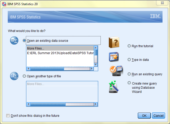
When SPSS is opened, an introductory dialog box pops up with a variety of different options including 'Open an Existing Data Source,' 'Open Another Type of File,' 'Run the Tutorial,' 'Type in Data,' and 'Create New Query Using Database Wizard.' This portion of the tutorial will explain each of these options. This portion of the tutorial will also demonstrate how to merge multiple SPSS data files into one file.
Open an Existing SPSS Data Source
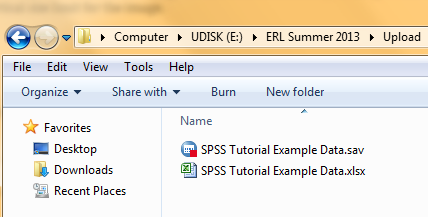
SPSS data files have the file extension *.sav. There are multiple ways to open an existing SPSS data file. One way to open an existing SPSS data file is to browse through the folders on your computer and double click on the desired file in the browse window. When an SPSS data file is opened this way, the introductory dialog box with file-opening options shown above will not pop up since a data file has already been selected.
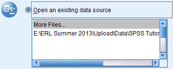
Another way to open an existing SPSS data file is to open SPSS, click the 'Open an Existing Data Source' option in the introductory dialog box, navigate to the location of the desired file on your computer in the browse window, and click OK.
To open an existing SPSS data file while the SPSS Data Editor window is open, click on the folder icon in the Data Editor Toolbar (below the main File toolbar) at the top of SPSS windows.

Open Another File Type
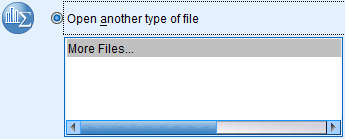
Data from other file types, such as excel files, can also be opened in SPSS. In order to open a data file that is not a *.sav SPSS file in SPSS, open SPSS, click the 'Open Another Type of File' option in the introductory dialog box, navigate to the location of the desired file on your computer in the browse window, and click OK. The contents of the file will be fit into the SPSS template.
Run the IBM SPSS Tutorial
The IBM SPSS tutorial included in the SPSS program is very detailed and informative. To access the IBM SPSS tutorial, open SPSS, click the 'Run the Tutorial' option in the introductory dialog box, and click OK.

You can also access the tutorial when data files are open and in use by clicking on 'Help' in the main toolbar at the top of the SPSS window and then by navigating to the 'Tutorial' option.

Type in Data
To create a new data file and type in your own variables and data values, open SPSS, click the 'Type in Data' option in the introductory dialog box, and click OK. This will open a new blank data editor window.

Merge Files
Data saved in multiple separate SPSS *.sav data files can be merged together into one data file. You can merge two files together to add cases or to add variables into your active file.
Please note that the images used in this example are from modified versions of the dataset attached to the table of contents of this tutorial.
To merge files, click on 'Data' in the main toolbar at the top of the SPSS data editor window. Select 'Merge Files...' and, in the side menu, you will be given the options of adding cases or adding variables.
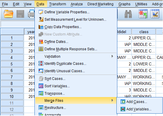
To add cases: Click on the 'Add Cases...' option in the 'Data-->Merge Files' side menu. Browse and select the file containing the data you wish to merge with your active file by clicking 'Browse' and then 'Continue' in the dialog box.
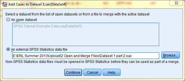
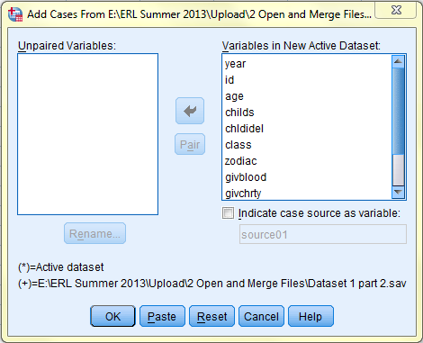
Then, in order to accurately merge cases, SPSS checks that the variables in the two files match. In the subsequent dialog box that pops up, variables from the dataset you wish to merge with your active dataset will be matched. Variables that match are automatically placed into the 'Variables in New Active Dataset:' field, and variables that do not match and that you do not wish to merge should be placed in the 'Unpaired Variables:' field. Upon clicking OK, all cases of each variable will be merged into your active dataset and are placed subsequent to all of the cases that were already in the file.
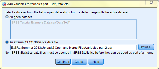
To add variables: Click on the 'Add Variables...' option in the 'Data-->Merge Files' side menu. Browse and select the file containing the data you wish to merge with your active file by clicking 'Browse' and then 'Continue' in the dialog box.
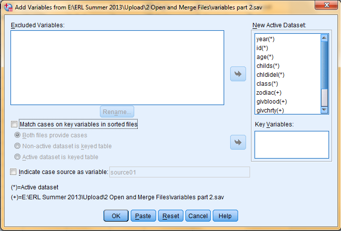
In the subsequent dialog box that pops up, variables from the dataset you wish to merge with your active dataset are listed in the 'New Active Dataset:' field. Variables that you do not wish to merge should be placed in the 'Excluded Variables:' field. Upon clicking OK, selected variables will be merged into your active dataset and are placed subsequent to all of the variables that were already in the file.
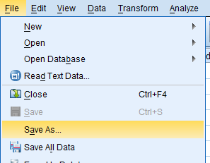
Files can be saved by clicking on 'File' in the toolbar at the top of SPSS windows and clicking 'Save' or 'Save As...'
Files can also be saved by clicking on the save icon in the Data Editor Toolbar below the main toolbar at the top of SPSS windows.

There are three different file types used in SPSS, each corresponding to one of the three SPSS windows:
Data files used in the data editor window are saved as *.sav files.
![]()
Output files used in the SPSS viewer are saved as *.spv files.
![]()
Syntax files used in the syntax editor (which is not included in the student version of SPSS and is not addressed in depth in this tutorial) are saved as *.sps files.
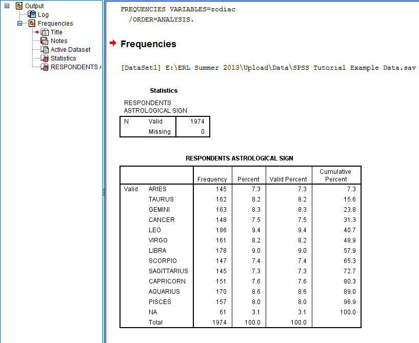
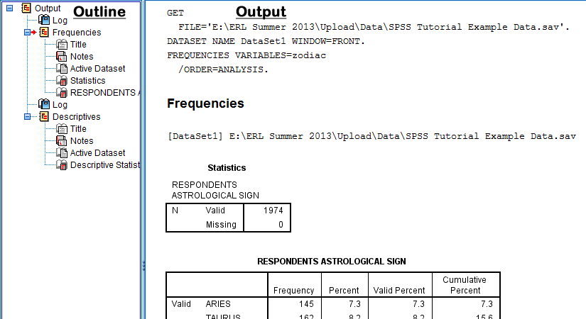
Output files in SPSS are displayed in the SPSS Viewer window which consists of two parts: an outline and output. The outline is on the left side of the the SPSS Viewer window, and the output is on the right side of the SPSS Viewer window. (In this example, the output will display the frequencies of respondents' astrological signs and descriptive statistics about the respondents' ages.)
Reading the Outline
The outline of the output, which is displayed on the left side of the SPSS Viewer window, presents an overview of the procedures and analyses that have been carried out. The outline presents this information in a standard way.
First, the outline lists that "Output" procedures are going to be presented. Then, the outline indents at each specific procedure that has been carried out. Each procedure is broken down into multiple parts on the outline, which correspond to the different items displayed in the output portion of the SPSS Viewer window: a log of the syntax used by SPSS to carry out the procedure, the type procedure, a title, space for pre-typed notes, the location of the active dataset from which the procedure was run, and statistical tables, charts, and graphs specific to each procedure. When an item is clicked in the outline, the corresponding output in the output section of the SPSS Viewer window is displayed and emphasized with a box and a small red arrow. For example, the following image displays the SPSS Viewer window when the frequency table for Respondents Astrological Sign is clicked in the outline:
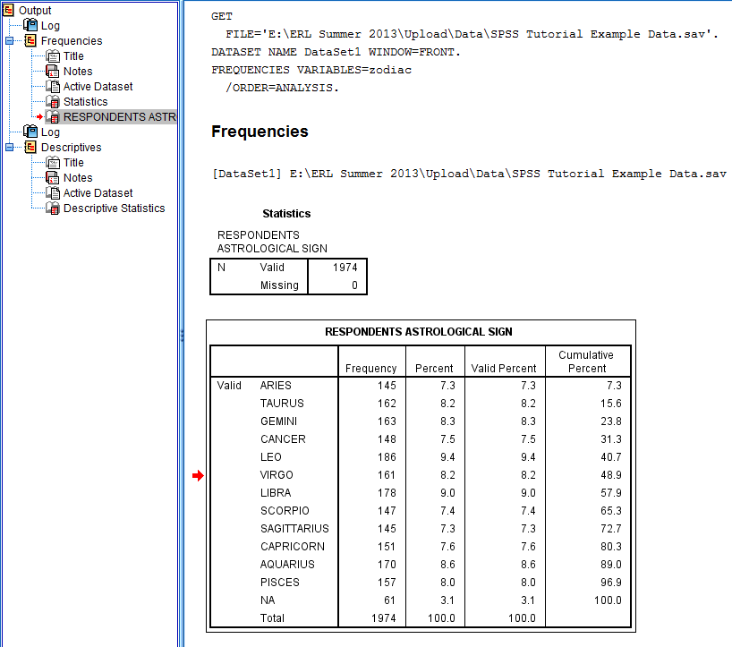
The outline can be widened by dragging the blue line separating the outline and the output to the right.
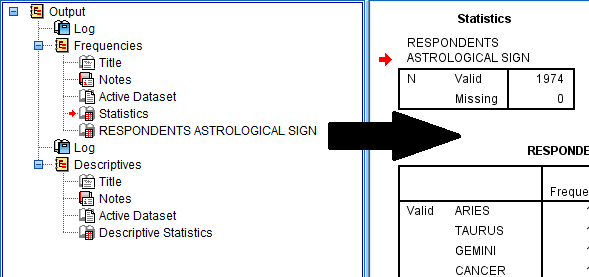
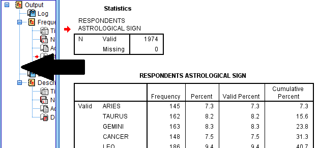
The outline can be and narrowed by dragging the blue line separating the outline and the output to the left.
The outline also serves as a collapsible and expandable index. The procedures and analyses listed in the outline can be minimized and collapsed or maximized and expanded.
To minimize an item in the outline, click on the little blue box with a minus sign which appears next to each procedure. Please note that when an item is minimized, it will not appear in the output portion of the SPSS Viewer window. It also will not appear on printouts.
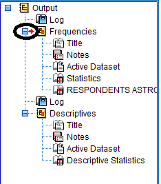
To maximize an item in the outline to make it appear in the output portion of the SPSS viewer window, click on the little blue box with a plus sign which appears next to procedures that have been minimized.
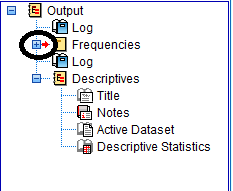
Reading the Output
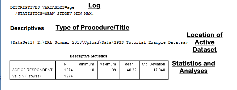
The output, which is displayed on the right side of the SPSS Viewer window, presents the procedures and analyses that have been carried out. The output presents this information in a standard way.
Each procedure is broken down into multiple parts that all correspond with the index of items in the outline portion of the SPSS Viewer window: a log of the syntax used by SPSS to carry out the procedure, the type procedure, a title, the location of the active dataset from which the procedure was run, and statistical tables, charts, and graphs specific to each procedure. When an item is clicked in the output, the corresponding item in the outline section of the SPSS Viewer window is highlighted and designated with a small red arrow.
Changing Titles
Titles in the outline and in the output can be changed by double clicking on the title you wish to change. However, please note that when you change the title in one location (either the outline or the output), the change is not reflected in the other. For example, if the title of the frequency table in the output is changed from 'Frequencies' to 'Frequencies of Astrological Signs,' the new title is not displayed in the outline.

Printing Output
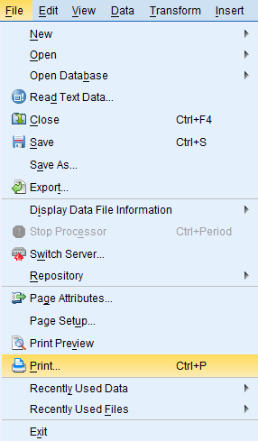
To print the output, click on 'File' in the toolbar at the top of the SPSS window, and then click 'Print...' from the dropdown menu.
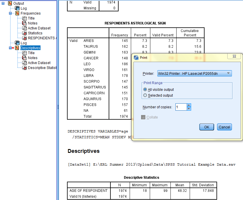
The dialog box that pops up gives the option of either printing 'All Visible Output,' which will print all procedures that are not minimized in the outline, or printing 'Selected Output,' which prints only the procedure selected in the outline. In the example below, All Visible Output is selected because I am interested in printing the entire output and not just the Descriptives procedure that is selected in the outline.
Add a Header/Footer to a Printout
To add a header or footer to a printout, click on 'File' in the toolbar at the top of the SPSS window, and then click 'Page Attributes' from the dropdown menu.
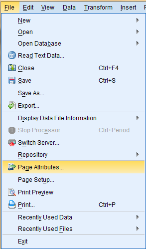
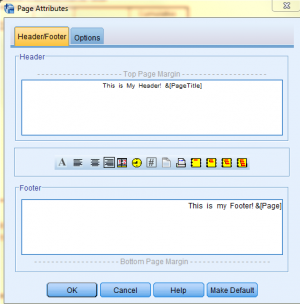
Then, in the Page Attributes dialog box, and type in your header and footer in their respective fields. Then click 'Print...'from the 'File' dropdown menu.
The Data Editor window is for entering variables and cases (data values). The Data Editor window has two views: a Data View and a Variable View. Click the tabs at the bottom left corner of the Data Editor window to toggle between the two views. When a view is selected, the corresponding tab turns yellow. This section of the tutorial provides instruction for how to use many of the functions of the Data Editor in both the Data View and the Variable View.
![]()
Entering Variables in the Data Editor
The Variable View of the Data Editor displays the names and qualities of every variable. Each row represents a single variable. The columns contain information about specific features of each variable such as the Name, Type, Label, and Value. These qualities will be discussed further below. The following image depicts the Data View of the sample data file that contains 15 variables (attached to the table of contents of this tutorial).

Qualities of Variables: Name, Type, Label, Value, etc...
The columns of the Data Editor contain information about specific features of each variable.
![]()
Name: Variable Names are short titles given to variables. Variable names can be up to a maximum of 64 characters. A longer and more descriptive variable label can be given to a variable in another column for a more descriptive name. All variable names are listed in the first column in the Variable View.

Variable names are important because they appear as column headings in the Data View.
![]()
However, variable names serve no other purpose. The SPSS default setting is for variable names to not show up in output, and, instead, the more detailed variable labels are displayed. However, this setting can be changed: Click on 'Edit' in the top toolbar, and then click 'Options' in the dropdown menu. Select the 'General' tab at the top of the dialog box that pops us, and then select your desired display option in the 'Variable Lists' field.
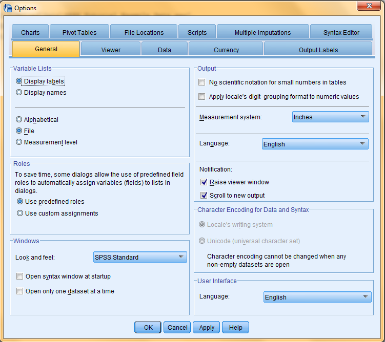
Type: The Type refers to whether the variable is in Numeric, Comma, Dot, Scientific notation, Date, Dollar, Custom currency, String, or Restricted Numeric (integer with leading zeros) format.
To change the variable Type from the default Numeric setting, click on the variable's Type cell. Then, click on the '...' box that appears on the right side of the cell.
![]()
In the dialogue box that pops up, select a variable Type, and click 'OK.'
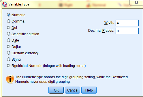
Width: The Width refers to the number of characters that can be entered as data values for the variable in the Data View. This number includes decimal places and the decimal point as well. Variable Width can be changed manually by clicking on the variable's Width cell and typing in a number. Please note: the width number must be larger than the number of Decimal places.
Decimals: The Decimals refers to the number of decimal points displayed in the Data View for each case value. The number of decimals can be changed manually by clicking on the variable's Decimals cell and typing in a number.
Label: Variable Labels are long, more descriptive titles given to variables in addition to the short variable names used to identify variables as the column headings of the Data View of the Data Editor. Variable Labels can be up to a maximum of 256 characters.
The SPSS default setting is for the detailed and descriptive variable Labels to be displayed in output instead of variable Names. However, this setting can be changed: Click on 'Edit' in the top toolbar, and then click 'Options' in the dropdown menu. Select the 'General' tab at the top of the dialog box that pops us, and then select your desired display option in the 'Variable Lists' field.

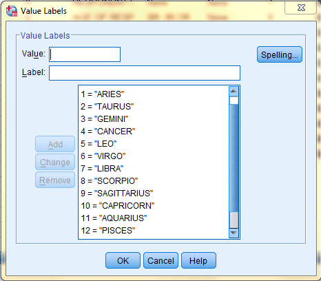
Values: Value Labels are textual labels that should be assigned to all nominal variables that represent different groups or categories with numbers. For example, in the variable 'zodiac,' the numbers 1-12 correspond with textual entries for each of the astrological signs. To add in Value labels, double click on the variable's Values cell, and then type in the Values and Labels in their respective fields.
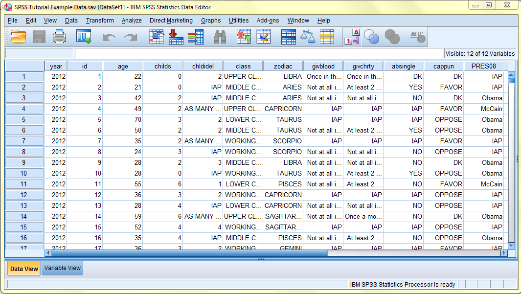
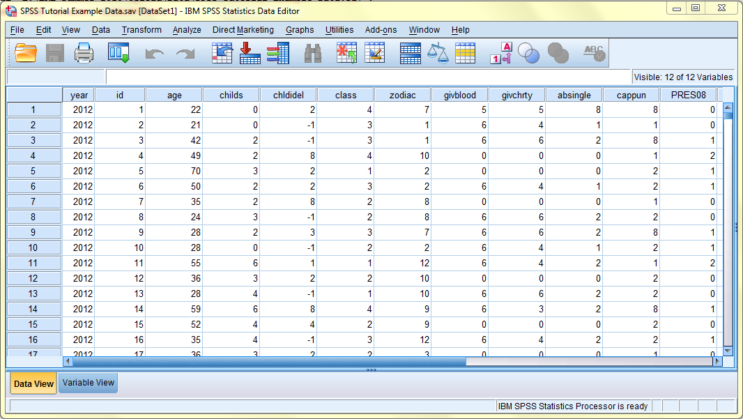
The SPSS default is to display nominal data in the Data View by Label and not by number, even if the data is typed in as numbers. (Specifically, the Data Editor will display the textual Values even if the data is typed in numeric form, which saves time from typing long text entries.) However, this default display setting can be changed by clicking on the 'Value Labels icon in the Data Editor toolbar when in the Data View of the Data Editor Window.
![]()
The following image displays the Data View with Value Labels turned on:
The following image displays the Data View with Value Labels turned off:
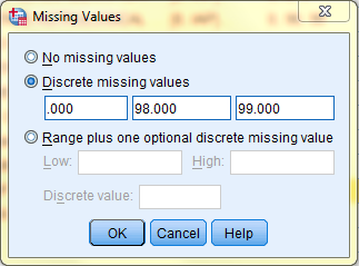
Missing: The Missing column allows users to define data as missing. This is useful when identifying different types of missing data such as data values that are missing because respondents ignore questions and data values that are missing because not all questions apply to all respondents. Missing data values are treated differently by SPSS and are excluded from most analyses. To define data as Missing, click on the variable's Missing cell and then click on the '...' box that appears on the right side of the cell.
![]()
Then, enter the missing data values in their respective fields in the dialog box that pops up. For example, the variable 'Number Of College-Level Science Courses R Have Taken' has the discrete missing values of 0, 98, and 99, because those values represent the responses of 'IAP' (inapplicable), DONT KNOW, and NO ANSWER, respectively.
Columns: The Column refers to the number of characters the column displays. This can be changed manually by clicking on the variable's Column cell and typing in a number or by clicking on and dragging the column borders. Please note that changing the column value changes only the display of the variable in the Data View and does not change the meaning of the variable itself.
Align: Align refers to how data values for the variable are aligned in the cells of the Data View. Data values can be left, right, or center justified. The SPSS default setting is right alignment. Alignments can be changed by clicking on the variable's Align cell and then clicking on the down arrow to access a dropdown menu of alignment options.

Measure: Measure is a way of further categorizing a variable's type as either ordinal, nominal, or scale. Measures can be changed by clicking on the variable's Measure cell and then clicking on the down arrow to access a dropdown menu of Measure options.

Role: Role denotes how SPSS will be using the variable. The SPSS default is to assign every variable the role of an 'input' variable that will be used for predictions.

Entering Cases in the Data Editor
The Data View displays every case and data value for all variables. Data values can be entered by clicking on a cell and typing in the value.
The columns in the Data View correspond with each variable, and each column heading displays a variable name.
![]()
The rows in the Data view represent individual data cases. Cases are identified by number and contain data values for each variable.

Select Rows/Columns
To select a single row, click on the row number.
To select a single column, click on the column heading.
To select an entire dataset, click on any cell within the dataset, then press Control and A on the keyboard at the same time, and the entire dataset will be selected.
To select multiple rows/columns, if the rows/columns are adjacent, click on the first desired row/column, then press and hold down the Shift button while clicking the last desired row/column. When you let go of the Shift button, the desired rows/columns will remain selected.
To select multiple rows/columns when the rows/columns are not adjacent, click on the first desired row/column, then press and hold down the Shift and Control buttons while clicking the remaining desired rows/columns. When you let go of the Shift and Control buttons, the desired rows/columns will remain selected.
View Grid Lines
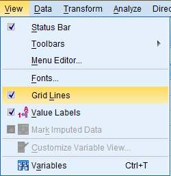
The SPSS default is for grid lines to be displayed in the Data Editor window. To change this setting, click on 'View' in the top toolbar, and then select or deselect 'Grid Lines' in the dropdown menu.
Change Grid Font
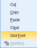
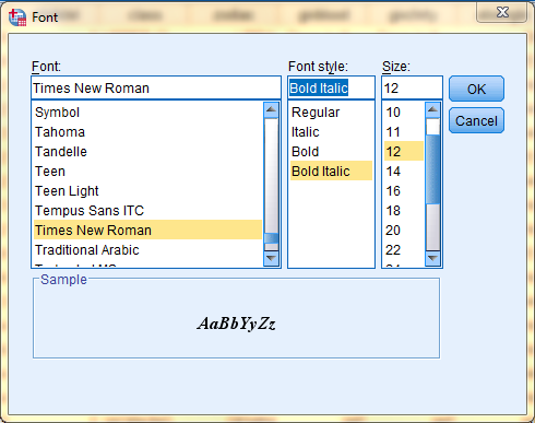
The SPSS default font is SansSerif, regular style, in size 10. To change this, right-click on any cell in the dataset, and then click 'Grid Font' from the dropdown menu that is displayed.
Then, in the dialog box that is displayed, select your desired font and click OK. Please note that Grid Font changes apply to the entire dataset and not to individual cells.
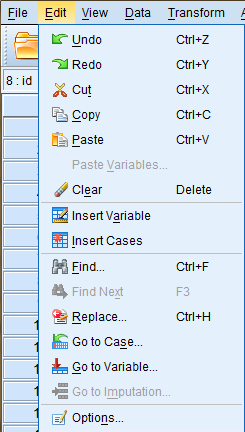
To access editing options in SPSS, you can use either the 'Edit' dropdown menu or the Data Editor Toolbar.
The 'Edit' dropdown menu can be accessed by clicking on the 'Edit' button in the top toolbar of the SPSS window. It contains many useful functions that will be discussed in depth in this portion of the tutorial.
Similarly, the Data Editor Toolbar, which appears under the top 'File' toolbar, contains many useful functions that will be discussed in depth in this portion of the tutorial.
![]()
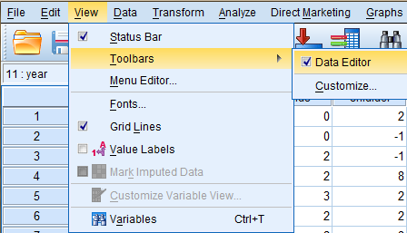
If the Data Editor Toolbar is not visible in your SPSS window, you can activate it by clicking 'View' and then 'Toolbars' in the dropdown menu. In the 'Toolbars' side menu, select 'Data Editor.'
Undo and Redo
The undo and redo functions can be accessed in the 'Edit' dropdown menu and also in the Data Editor Toolbar. You can undo/redo the actions performed on the most recently edited items in reverse chronological order.
![]()
Cut, Copy, Paste
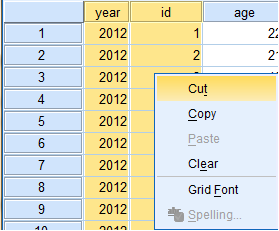
The cut, copy, and paste functions can be accessed in the 'Edit' dropdown menu and also by right-clicking on the highlighted data field to which you are applying these functions.
Clear
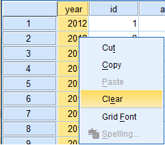
'Clear' is used to delete highlighted items. The clear function can be accessed in the 'Edit' dropdown menu and also by right-clicking on the highlighted data field to which you are applying this function.
Insert variable, Insert cases
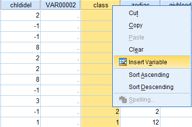
'Insert...' adds a blank row (case) or column (variable). The insert function can be accessed in the 'Edit' dropdown menu and also in the Data Editor Toolbar.

Rows (cases) and columns (variables) can also be inserted by right-clicking on the row or column name directly below or directly to the right of where you wish to insert the case/variable.
Find, Replace
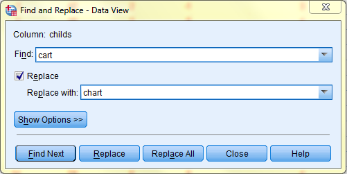
Find and Replace are search functions. If searching with 'Replace,' you will be given the option of replacing the items found in the search with whatever you enter into the 'Replace with' field. The 'Find' and 'Replace' functions can be accessed in the 'Edit' dropdown menu
Go to Case, Go to Variable
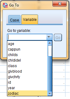
'Go to Case' and 'Go to Variable' are methods of maneuvering through large data files to find specific data values quickly. Both 'Go to...' functions can be accessed in the 'Edit' dropdown menu and also in the Data Editor Toolbar.

When you use either of the 'Go to...' functions, a dialog box containing a dropdown menu of all cases/variables pops up, allowing for quick access to cases/variables.
Options
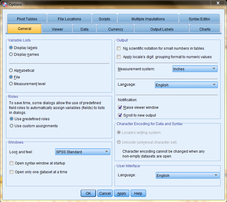
More options can be accessed by clicking 'Options' in the 'Edit' dropdown menu. The Options dialog box that pops up has many tabs that each contain many different options fields.
In SPSS, variables can be transformed into new variables while preserving the original data. This is particularly useful when recoding data, doing score reversals, and when computing mathematical manipulations of variables such as complex summations.
Recoding Variables
In SPSS, variables can be recoded either into the same variable, which overwrites the original data values, or into a different variable, which does not overwrite the original data values and creates a new variable in a new column. Recoding into a different variable is highly recommended in case you need to access the original data in the future.
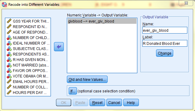
In this example, the 'givblood' variable, which presents information regarding how often respondents have given blood within the past year, will be recoded into a new variable that presents how many respondents have given blood at least once within the past year, with 0 meaning the respondent has not given blood within the past year and 1 meaning the respondent has given blood at least once within the past year.
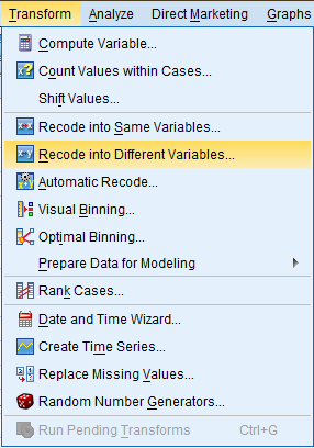
To recode variables, click 'Transform' in the toolbar at the top of the SPSS window, and then click 'Recode into Different Variables' in the dropdown menu.
Then, in the dialog box that pops up, select the variable you would like to transform (the 'givblood' variable), and double click on it to bring it to the 'Numeric Variable --> Output Variable:' field. Then, in the 'Output Variable' field, enter the name and label you would like to give to the new variable. Next, click on 'Old and New Values.'
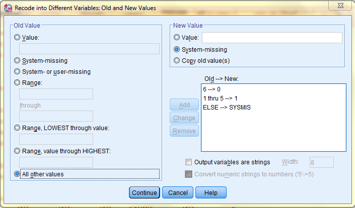
Upon clicking 'Old and New Values,' a dialog box pops up. This dialog box enables you to recode all data values individually or in a range. First, in the 'Old Values' field, select whether you are recoding a specific value or a range of values and then enter the specific value or range of values in its field. Then, in the 'New Values' field, select the 'Value' button and type in the new data value. Lastly, click 'Add.' When all data values have been recoded and added, click 'Continue.'
In this example, 6 is redoded into 0, because, in the original variable, 6 represents respondents who have not given blood within the past year. Then, 1 through 5 are recoded into 1 because, in the original variable, all of these values respresent respondents who have given blood at least once within the past year. Lastly, 'All other values' is selected in the 'Old Values' field and is recoded in the 'New Values' field into 'System-missing' data because all other values represented respondents who were not asked whether they had given blood, respondents who answered that they did not know, and respondents who did not answer at all.
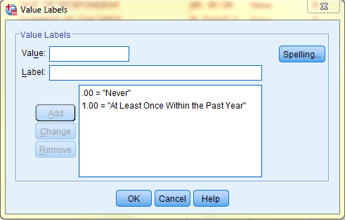
Lastly, in the Variable View of the Data Editor, value labels must be given to the new variable because value labels should be assigned to the values of all numeric nominal variables that represent different groups or categories with numbers. To add in value labels, double click on the variable's Values cell, and then type in the Values and Labels in their respective fields.
In this example, 0 is labeled as 'Never' because it represents respondents who have not given blood within the past year, and 1 is labeled as 'At Least Once Within the Past Year' because it represents respondents who have given blood at least once within the past year.
The new variable is now complete and added to the dataset.
![]()
Mathematical Manipulations to Create New Variables
Variables in SPSS can be mathematically manipulated to create new variables while preserving the original data.
In this example, the variables 'childs,' each respondent's number of children, and 'chldidel,' each respondent's ideal number of children, will be manipulated to create a new variable, 'diff_in_num_children,' which represents the absolute value of the difference between each respondent's actual number of children and ideal number of children.
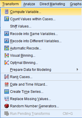
To mathematically manipulate variables, click 'Transform' in the toolbar at the top of the SPSS window, and then click 'Compute Variable' in the dropdown menu.
Then, in the Compute Variable dialog box that pops up, enter the name of your new variable, 'diff_in_num_children,' in the 'Target Variable' field. Then, click 'Type & Label' to give your new variable a Label(Difference Between Ideal Number of Children and Actual Number of Children) and Type (Numeric) in the dialog box that pops up, and click continue. Next, select the desired function group from the 'Function group' field (Arithmetic) and then the desired specific function from the 'Functions and Special Variables' field (Abs). Lastly, fill in the mathematical manipulation in the 'Numereic Expression' field by adding variables from the variable list and mathematical functions from the functions box. Click 'Continue.'
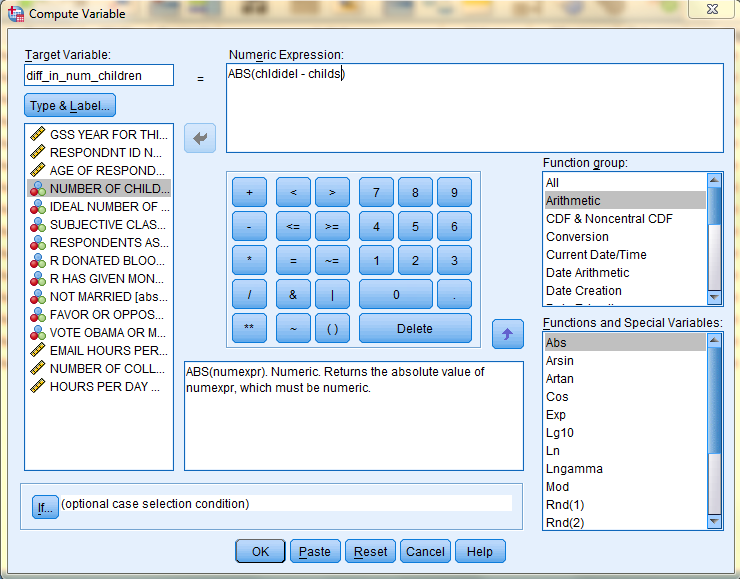
The new variable, 'diff_in_num_children,' with its corresponding newly calculated data values, will be added to the Data Editor. The image below displays the new variable in the Variable View
![]()
Binning Variables
Binning is a method of grouping scaled data into intervals.
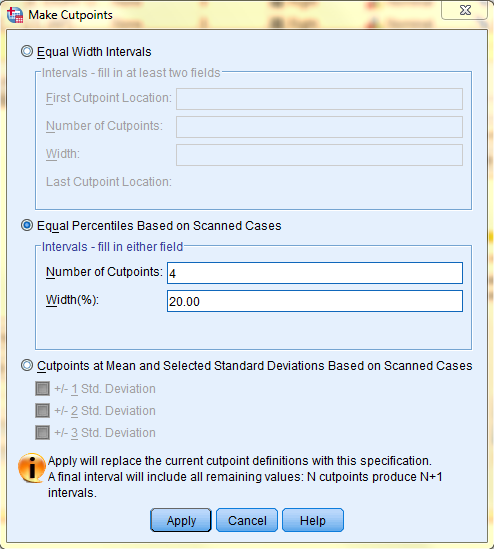
In this example, the scaled variable 'Age' will be binned into 5 intervals of equal size to enable statistical comparisons between, for example, the youngest 20% and oldest 20% of the respondents.
To bin a variable, click 'Transform' in the toolbar at the top of the SPSS window, and then click 'Visual Binning...' in the dropdown menu.

Then, in the dialog box that pops up, select the desired variable from the 'Variables' field and then double click on it to bring it to the 'Variables to Bin' field, and click 'Continue.'
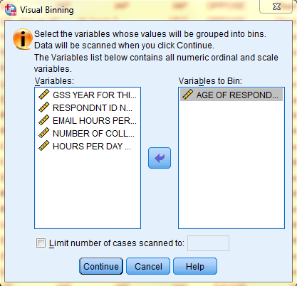
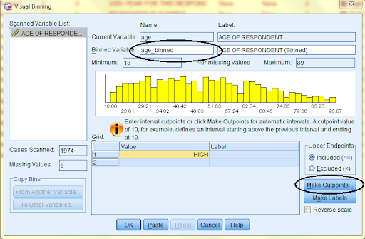
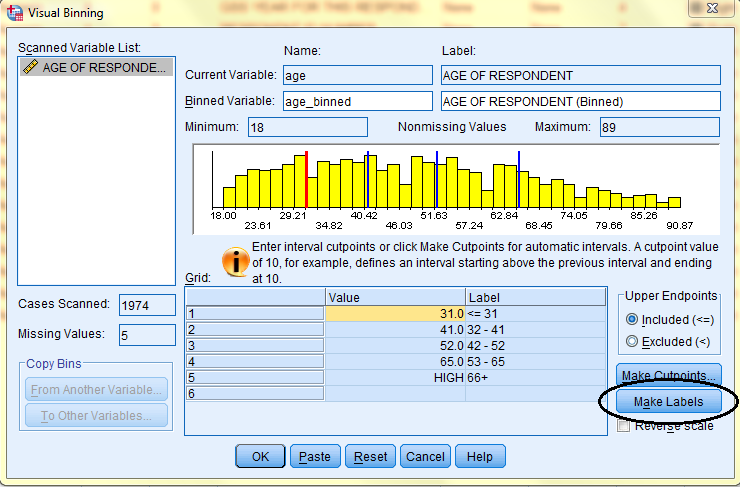
In the dialog box that pops up, information about the entire dataset will be displayed, such as the minimum and maximum data values. In the Binned Variable Name field, enter the name of the new binned variable (age_binned). Then, click 'Make Cutpoints' to create the cutpoints of the intervals.
In the dialog box that pops up, select the desired cutpoint option and type in the appropriate values. Then, click 'Apply'. Here, we selected 'Equal Percentiles Based on Scanned Cases' and specified for 4 cutpoints to make 5 intervals that each reflect 20% of the data. (Please note that n cutpoints yields n+1 intervals.)
Back in the Visual Binning dialog box, cutpoint values will be displayed. Then click 'Make Labels,' and corresponding value labels will automatically be created. Then, click OK.
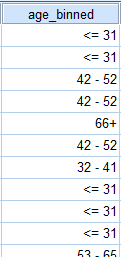
The new binned variable will be added to the Data Editor. The following image displays the 'age_binned' variable in the Data View of the Data Editor with value labels turned on.
Data in SPSS can be sorted and filtered in a variety of ways.
Sort Data
Columns of data in the Data View of the Data Editor window can be sorted in ascending or descending order.
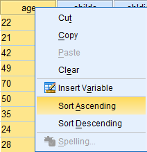
To sort data, right click on the column heading (the name of the variable you wish to sort) and click on the desired sort order (ascending or descending). The variable will be sorted along with each case's corresponding data values in the other variable categories.
Select Cases: Filter
The Select Cases function in SPSS enables users to select specific cases of data according to a variety of user-specified conditions. This is useful when focusing on subgroups within a dataset.
Filter According to One Condition:
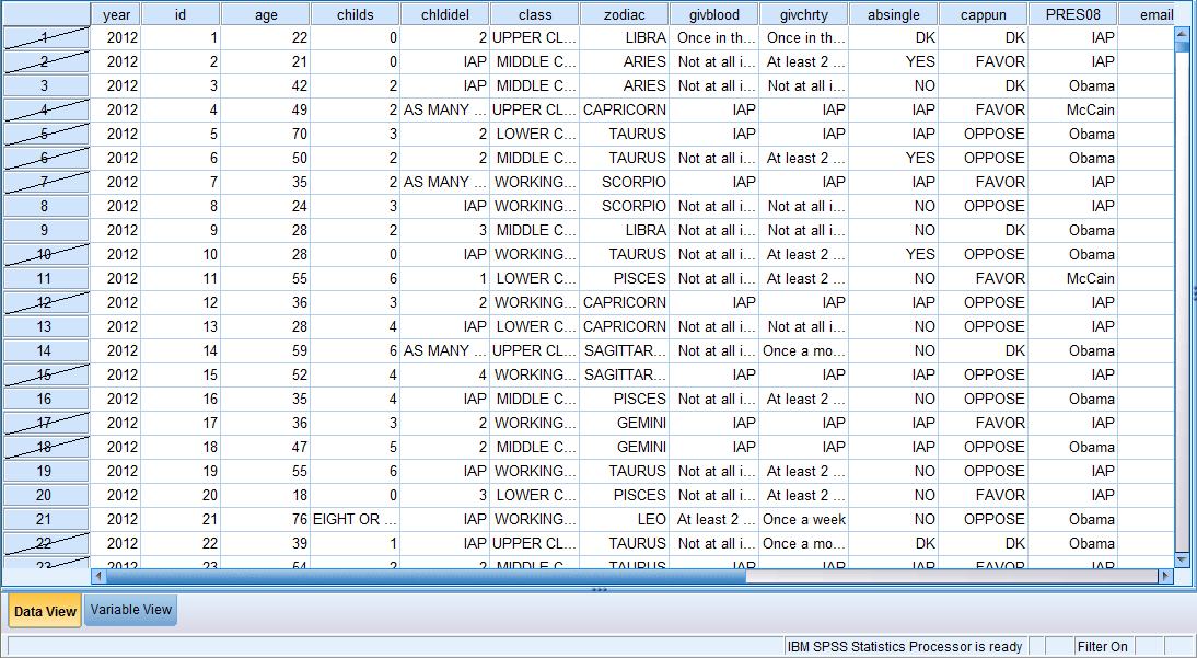
In this example, we want to select data from respondents who are married and filter out all other data. Specifically, if the variable absingle = 2, then the data from respondents who are married will be selected, because 2 represents respondents who are married. All other cases will be filtered out. When cases are selected and other data is filtered out, all further analyses and graphs reflect only the selected data (until the filter is turned off).
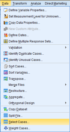
To use the Select Cases function, click on 'Data' in the toolbar at the top of the Data Editor window, and then click on 'Select Cases' in the dropdown menu.

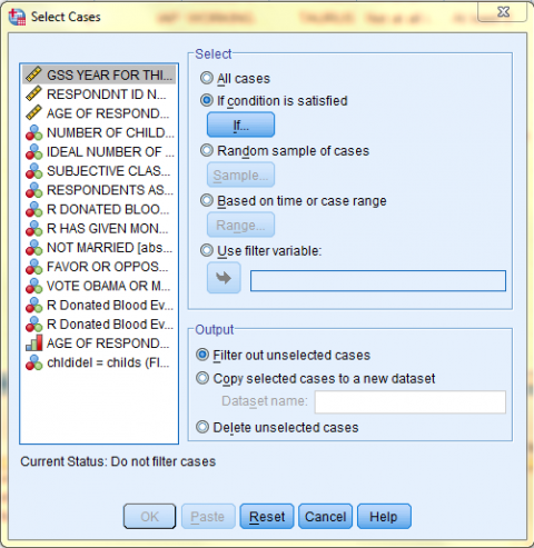
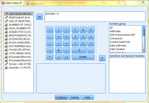
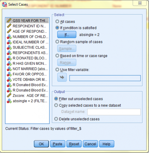
In the dialog box that pops up, the 'Select' field offers a few different methods of filtering data. In the 'All cases' option, all data cases are selected and none are filtered out. In the 'If condition is satisfied' option, data is filtered out in accordance with a predetermined condition. Select the 'If condition is satisfied' option and click 'If...' to specify the filtering conditions. For example, if you are interested in respondents that are married, then you would want to select those cases. In our dataset, marital status is denoted by the 'absingle' variable, and marriage is denoted with a 2. Hence, the specific condition is: absingle = 2.
In the Select Cases: If dialog box that pops up, enter the specific conditions according to which you would like data to be selected and filtered. Then, click 'Continue.' In this example, the specific condition is: absingle = 2. All cases where the respondent is married will be selected, and all other cases will be filtered out.
Back in the Select Cases dialog box, the If Condition is now displayed next to the 'If...' button. Next, choose your desired output option and click 'OK.' In this example, we want to 'Filter out unselected cases.'
The following image displays the Data View of the Data Editor with the 'absingle = 2' filter on. Note how the bottom right corner of the screen says 'Filter On.' Remember, all further analyses and graphs will reflect only the selected data (until the filter is turned off).
To turn the filter off, click on 'Data' in the toolbar at the top of the Data Editor window, and then click on 'Select Cases' in the dropdown menu. Then, click on 'All cases' to deselect the 'If condition is satisfied' option, and click 'OK'.
Filter According to Multiple Conditions:
In this example, we want to select data from respondents who are in the middle class or upper class and above the age of 50, and we want to filter out all other data. Specifically, if the variable 'class' is equal to 3 or 4, and the variable 'age' is greater than or equal to 50, then the data will be selected (because the 'class' values 3 and 4 correspond with respondents who are in the middle and upper class, and the 'age' values greater than or equal to 50 correspond with respondents who are 50 years old and above. All other cases will be filtered out. When cases are selected and other data is filtered out, all further analyses and graphs reflect only the selected data (until the filter is turned off).
To use the Select Cases function, click on 'Data' in the toolbar at the top of the Data Editor window, and then click on 'Select Cases' in the dropdown menu.
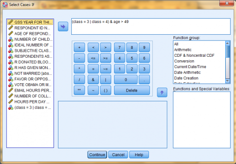
In the dialog box that pops up, the 'Select' field offers a few different methods of filtering data. In the 'All cases' option, all data cases are selected and none are filtered out. In the 'If condition is satisfied' option, data is filtered out in accordance with a predetermined condition. Select the 'If condition is satisfied' option and click 'If...' to specify the filtering conditions. For example, if you are interested in respondents who are in the middle or upper class and are above the age of 49, then you would want to select those cases. In our dataset, class is denoted by the 'class' variable, and the 'class' values 3 and 4 correspond with respondents who are in the middle and upper class. Age is denoted by the 'age' variable, and the 'age' values greater than 49 correspond with respondents who are 50 years old and above. Hence, the specific condition is: (class = 3 | class = 4) & age > 49.

In the Select Cases: If dialog box that pops up, enter the specific conditions according to which you would like data will be selected and filtered. Then, click 'Continue.' In this example, the specific condition is: '(class = 3 | class = 4) & age > 49.' All cases where the respondents are in the middle or upper class and are above the age of 49 will be selected, and all other cases will be filtered out.
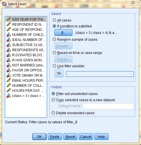
Back in the Select Cases dialog box, the If Condition is now displayed next to the 'If...' button. Next, choose your desired output option and click 'OK.' In this example, we want to 'Filter out unselected cases.'
The following image displays the Data View of the Data Editor with the '(class = 3 | class = 4) & age > 49' filter on. Note how the bottom right corner of the screen says 'Filter On.' Remember, all further analyses and graphs will reflect only the selected data (until the filter is turned off).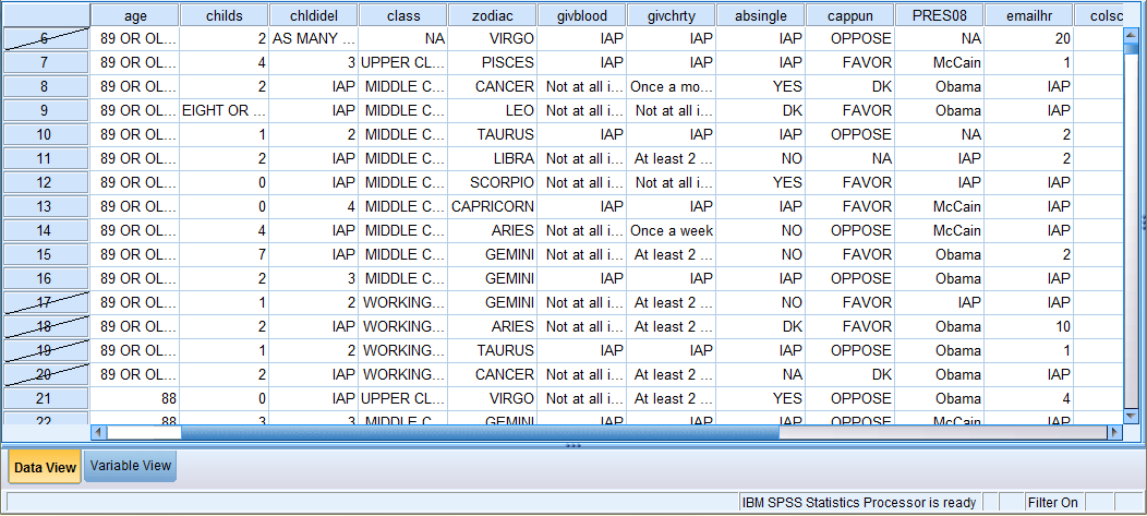
To turn the filter off, click on 'Data' in the toolbar at the top of the Data Editor window (specifically in the Data View), and then click on 'Select Cases' in the dropdown menu. Then, click on 'All cases' to deselect the 'If condition is satisfied' option, and click 'OK'.
Lastly, SPSS can filter a 'Random sample of cases,' cases 'Based on time or case range,' or based on a filter variable (filter variables are created each time a filter is made using any of the other filter options).
Split File
The Split File function in SPSS enables users to sort data and organize output by subgroups. This is useful when comparing data among groups.
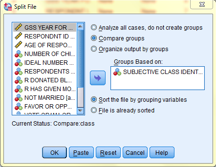
In this example, we will split the file (and all output) according to respondents' subjective class identification. Spefically, when a frequency table is generated, six individual frequency tables will be in the output, one for each class group (Lower, Working, Middle, Upper, DK, and NA).
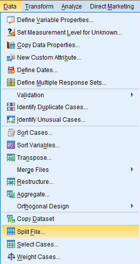
To use the Split File Cases function, click on 'Data' in the toolbar at the top of the Data Editor window, and then click on 'Split File' in the dropdown menu.
In the Split File dialog box that pops up, a few different methods of splitting data are offered. In the 'Analyze all cases, do not create groups' option, all data cases are selected and the file will not be split. This is the default. In the 'Compare groups' and 'Organize output by groups' options, data is split according to the groups (categories) of the categorical variable entered into the 'Groups Based on:' field. After selecting the desired split option, enter the desired categorical variable (Subjective Class Identification) into the 'Groups Based on:' field. Then, select 'Sort the file by grouping variables,' and click 'OK.'
The following image displays the Data View of the Data Editor split by 'class.' Note how the bottom right corner of the screen says 'Split by class.' Remember, all further analyses and graphs will reflect data split according to each class group (until the filter is turned off). For example, when a frequency table is generated, six individual frequency tables will be in the output, one for each class group (Lower, Working, Middle, Upper, DK, and NA).
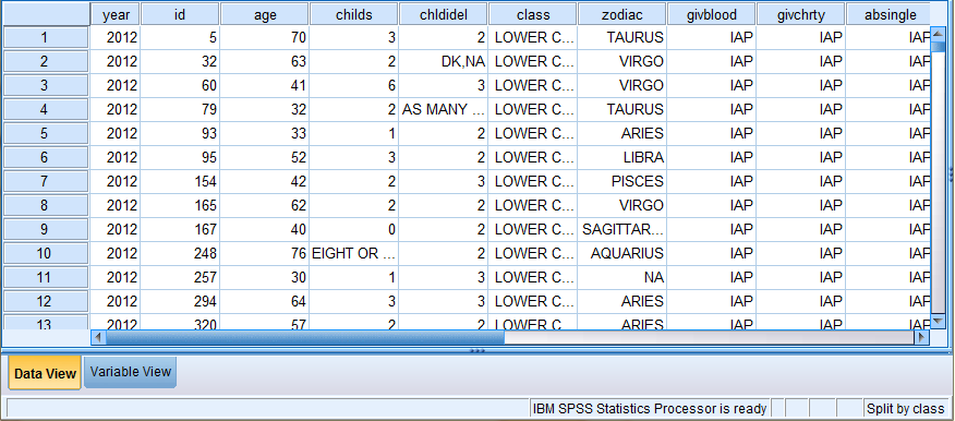
To turn the split off, click on 'Data' in the toolbar at the top of the Data Editor window (specifically in the Data View), and then click on 'Split File' in the dropdown menu. Then, click on 'Analyze all cases, do not create groups' to deselect the 'Compare groups' option, and click 'OK.'
Next: Descriptive Analysis