Formulas & Functions

Getting Started

Formulas and functions differ in Excel by one key feature. Formulas are written by you and functions pre-exist in the program. They have many similarities, as you will see in this page and the following ones covering formulas and functions. 

Here are some basic things to know about writing formulas in Excel. 

ALL formulas and functions must begin with an '='. No 'equals' equals no function! (or formula!)

Basic mathematical operators that you can use when writing a formula are:

*   for multiplication
/    for division 
+   for addition
-    for subtraction

The use of these operators follows the basic order of operations: *, /, +, - (muliplication, division, addition, subtraction). You can use ( ) parentheses if you would like operations completed in a different order (e.g. to add two numbers before multiplying them by another number: put the parentheses around the summation).

Writing Formulas

To get practice writing a formula, let's return to the dataset from the U.S. Census in 2010 and let's assume that the information for percent change between 2000 and 2010 was missing (or hadn't been provided).

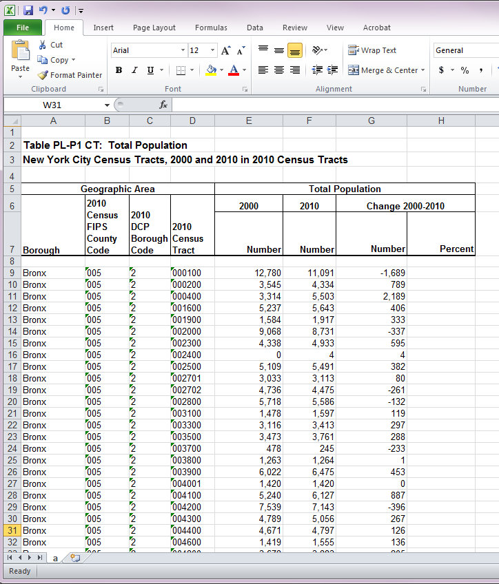
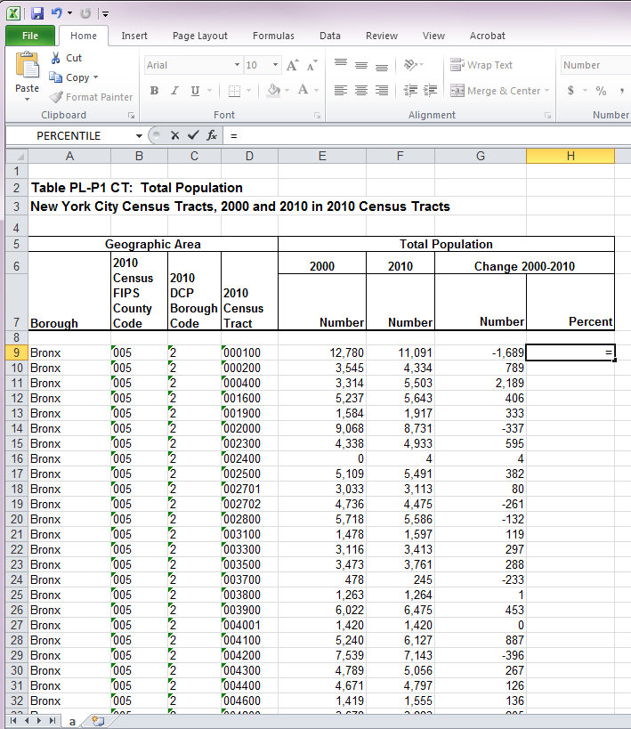
To write a formula, first click on the cell where you want the output to be. Then type '='.

You'll see the '=' in both the cell in which you are typing and in the formula bar. We could type "-1689 / 12780 * 100" following the '=' sign and this would give us the correct result, however, I'm just going to tell you flat out that you don't want to do that.

By writing the actual numbers into your function you are making Excel no better than a calculator, but there are a lot of ways that Excel can save you time and save you from making mistakes, if you use it well. So instead of typing the actual numbers, you want to select the cells that contain the numbers. You can do this by clicking on the cell with the mouse OR by typing the cell number/letter reference. 

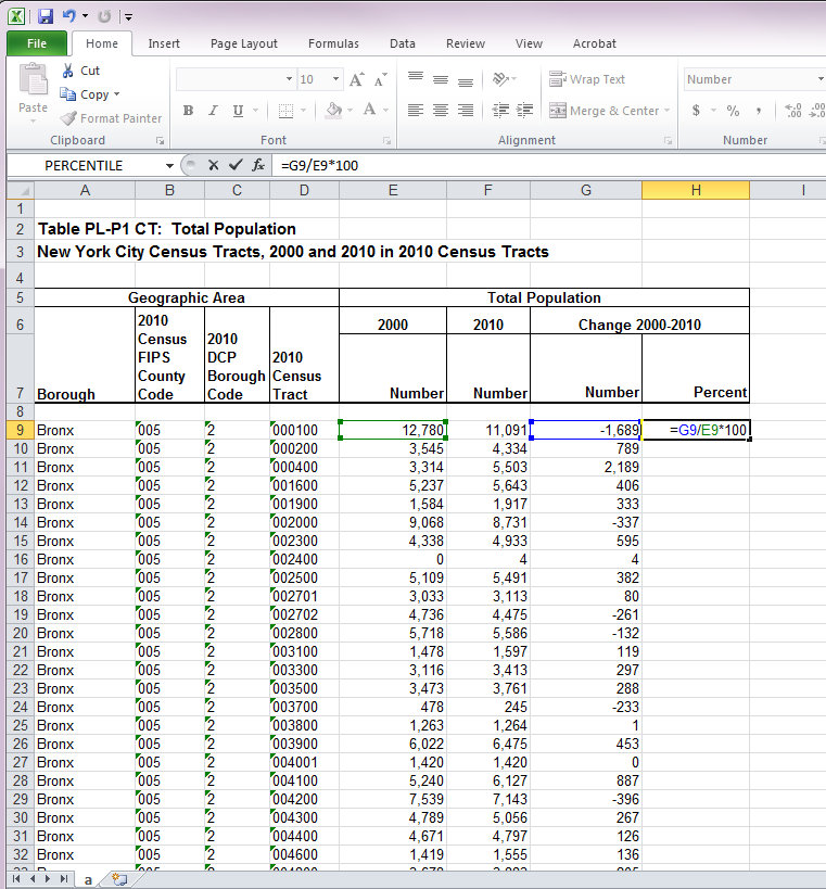
You'll see that the selected cells are color coded and that the colored cell number/letter references are referring to the cells that are outlined in the same color. This can make finding a cell used in a formula (or function!) easier when scanning a large dataset. Also, actual numbers remain black (like the *100). When you are done entering the function, press ENTER.

Using Cell Referents

It is important to use the cell referents instead of the actual numbers in case the numbers in the cells change. In this particular case, that shouldn't happen because this is a collected Census data and it would be unnecessary (not to mention inappropriate and unethical) to change it. However, you could be managing a budget or designing an experiment and would like to test how different values will affect the total outcome- then you will be very pleased to be able to change numbers in cells without having to rewrite your formulas!

Referencing a cell in another worksheet

If you are working with multiple worksheets, you might want to refer to a cell in Sheet2 while you're working Sheet1. Let's use a simple summation as an example. To add up the value of C2 in your current worksheet and the value of C2 in Sheet2, simply type:

=C2+Sheet2!C2

Using Auto Fill with Formulas

Another reason it is important to use the cell referents instead of typing the number is because we can repeat a formula (and a function) using Auto Fill instead of typing each iteration. Need a refresher on Auto Fill?

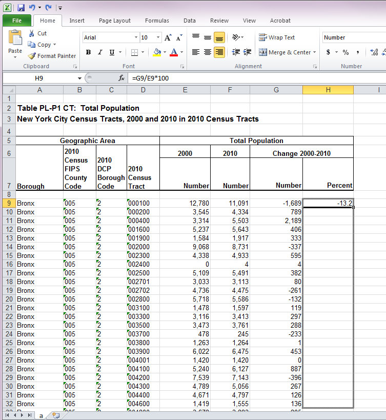
By using Auto Fill all of the selected cells now contain the formula. Notice that the formula changes for each cell it is copied into. The formula in H10 refers to the information in cells for G10 and E10, whereas our original formula in H9 referred to information in cells in G9 and E9. 

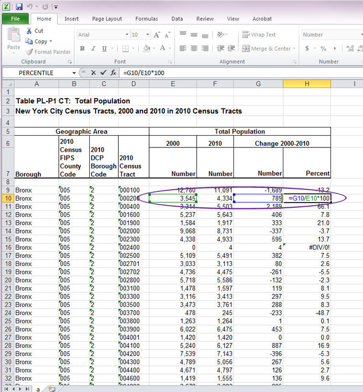
This is great when we want all of the referents in a formula to change, but it isn't so great when we don't want them all to change. (If you are concerned about what's going on in cell H16, you can jump to it here, or you can continue along and get to it after a page or two...)

Relative VS Absolute Referencing

As just mentioned, when using Auto Fill the formula changes referents so that each new entered formula refers to different cells. This is called relative referencing, but there are times when you do not want the cell referents to change when copying the formula into a new cell.  You can change the formula to have absolute referencing in which a particular cell will always be referred to in the function. 

Let's work through an example. So let's say, instead of typing 100 into the formula, we typed it into a single cell and referenced it in the formula. Our new formula in H9 would look like this.

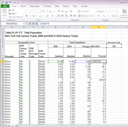
But if we used Auto Fill as before, the cells will look like this. 

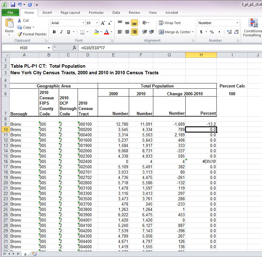
Do you know why we get one correct output and then the rest of the cells have zeros? Double check your thinking here. 

But we want the formula to always refer specifically to cell I6 since that is where we typed 100. To create an absolute reference we use the '$' inserted before the column letter, the row number, or both. What the '$' precedes will not change. So if we always want to reference column I, but change the row number, then the '$' should only precede the column letter. However, if we want the columns to change, but not the rows, the '$' should precede (have you got it?) the row. And if we want neither the column letter nor the row number to change (we want to always refer to a specific cell no matter what) the '$' should go in front of both the column letter and row number. 

To edit a formula in a cell, double click on the cell. This will allow you to edit the formula in the formula bar or in the cell itself. You can also single click on the cell and edit the formula in the formula bar. Just be aware that if you are editing the cell itself, the arrow keys will not navigate within the cell, but will navigate to adjacent cells. 

In our particular case, it is a specific cell that we don't want to change, so we could put the '$' in front of both the column letter and row number. 

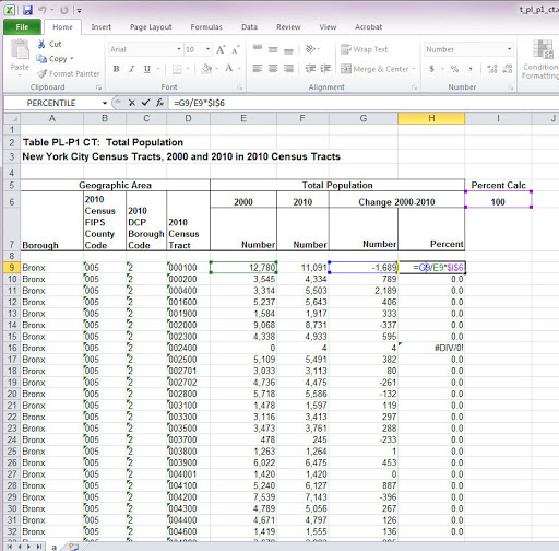
Then when we Auto Fill the rest of the cells, they are always multiplied by I6.

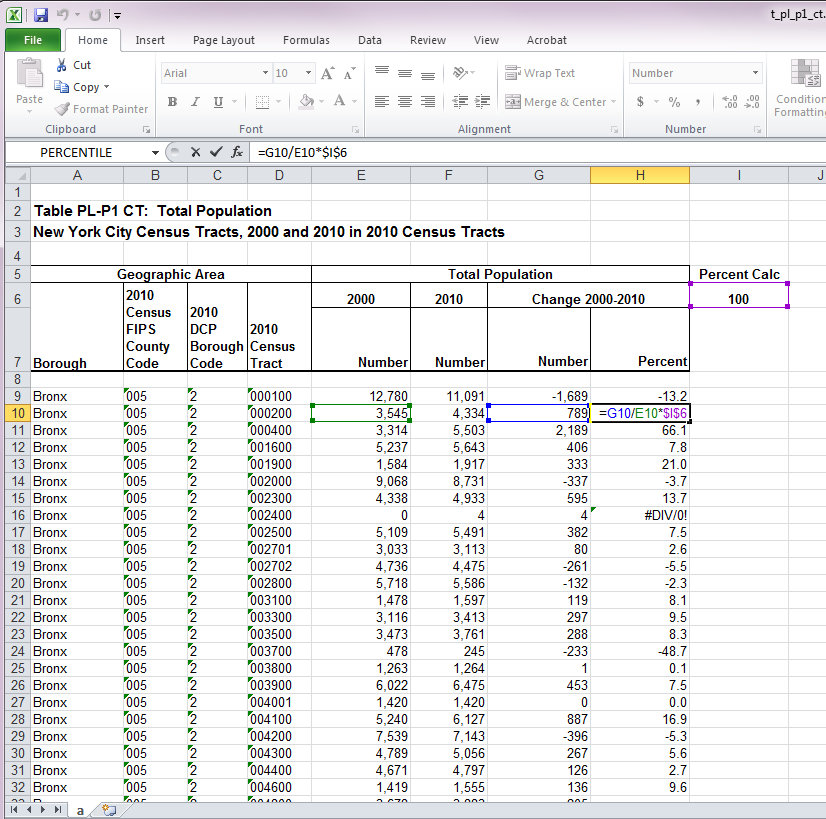
However, if we put the '$' only in front of the column letter, our output would look the same as before:

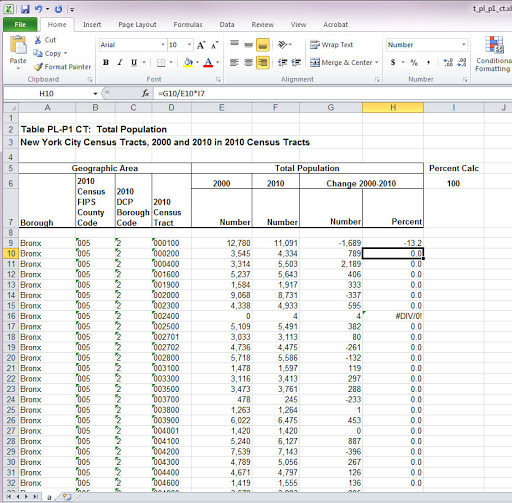
This is because the row numbers are not absolute and will change. If our Auto Fill were occurring horizontally rather than vertically, then the row number would not change, even if it were a relative reference but the column letter would.

Additionally, because we are calculating the percent change vertically (we are NOT dragging the Auto Fill horizontally), we could get away with putting the '$' only in front of the row number instead of putting it in front of both. 

I encourage you to play around with absolute and relative references to get a sense of when each is most useful or contact us if you have questions.

Function Basics

Excel has a library of functions that allows you to quickly make specific calculations. Functions in Excel take arguments. Most functions will require at least one argument. Arguments can be a range of data, a specified output, or other parameters, depending on the particular function. Arguments are typically presented in parentheses following the function.

Here are a number of common functions that you are likely to use: 

• Average(number1, number2) - calculates the average (mean) of a range of cells
• Stdev(number1, number2) - calculates the standard deviation of a range of cells
• Sum(number1, number2) - adds all of the values of a range of cells
• Count(value1, value2) - counts the number of items in a range of cells (blank cells will not be counted & neither will cells that are formatted as text)
• Median(number1, number2) - calculates the median of a range of cells
• Mode(number1, number2) - calculates the mode of a range of cells
• Max(number1, number2) - gives the maximum value of a range of cells
• Min(number1, number2) - gives the minimum value of a range of cells
• If(logical_test, value_if_true, value_if_false ) - allows one to perform a logical test (e.g. IF A1 >= 5, then 0 if true, or else 1 if false)

This is not an exhaustive list, by any means. We'll talk more about finding functions in the section below, (which you can jump to here) but first we should go over how to use functions in Excel.

Inserting a Function

For example, let's say you wanted to take the average of the increase in population of the first ten census tracts which you would need some sort of logical argument for doing (such as demonstrating a function for a tutorial). Click on the cell where you want the average to appear. Type '=' (because without an 'equals,' the function won't run), then type average, and then the open parenthesis. Excel will prompt you for the arguments. 

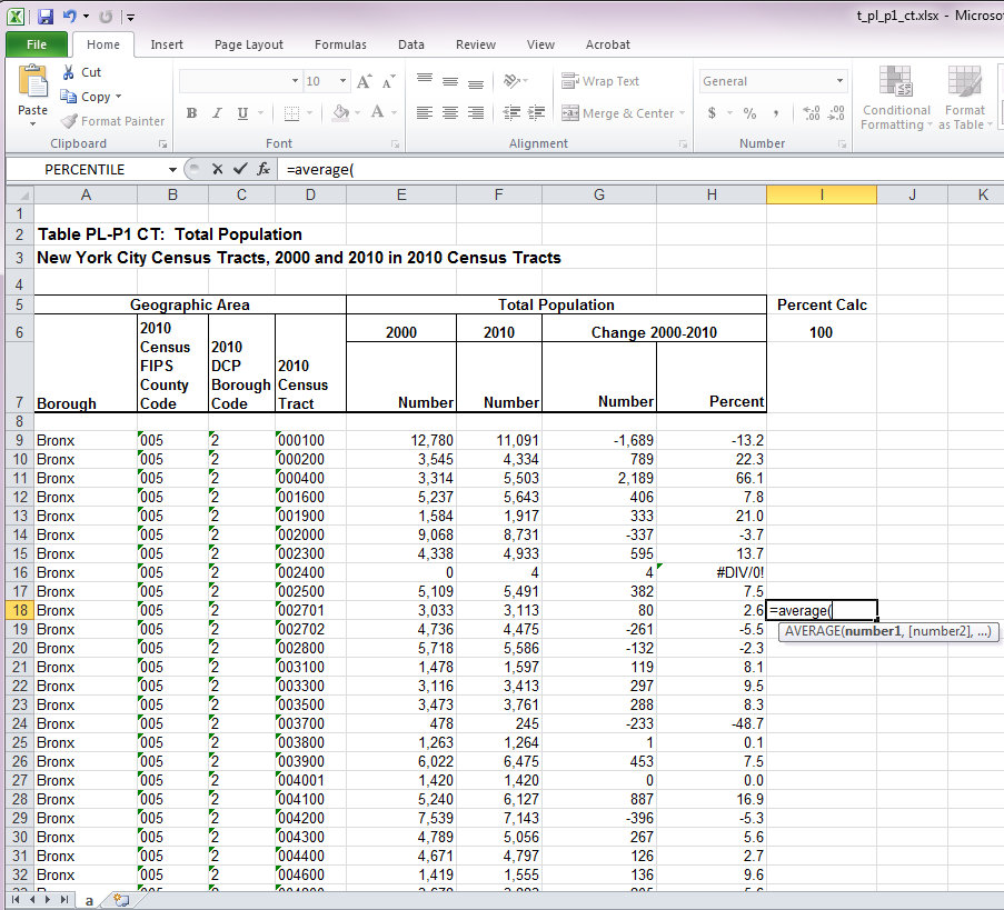
The required arguments are specified as 'numbers', however you can also use cell referents, so long as the cells are formatted as Number or General. The square brackets [ ] around an argument mean that the argument is optional. For the average function you must have at least one cell referent (or number) to average (of course, the average of a single value isn't very interesting- what's the point of calculating it really?). When entering arguments you can enter each one and separate them with a comma, as the argument list is presented below. This would be quite time consuming if you have a ton of numbers to average. You can also select the entire range of cells that you want to average with the mouse.

You can also type "G9:G18" if you prefer to remain at the keyboard instead of switching back and forth between the keyboard and the mouse. 

In the formula bar we see the function and in the cell we see the output. Let's walk through another example using the sum function.

Excel Functions: Sum Example

For example, let's say a small grocery store (or maybe your local bodega) was interested in how much customers spent on eggs and milk each day in a given week. After setting up the headers...

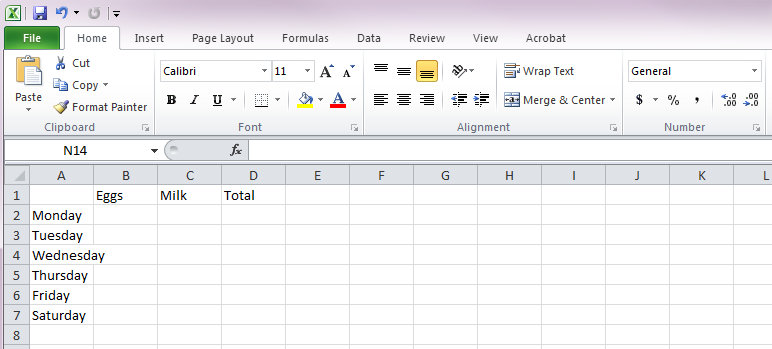
Insert the data.

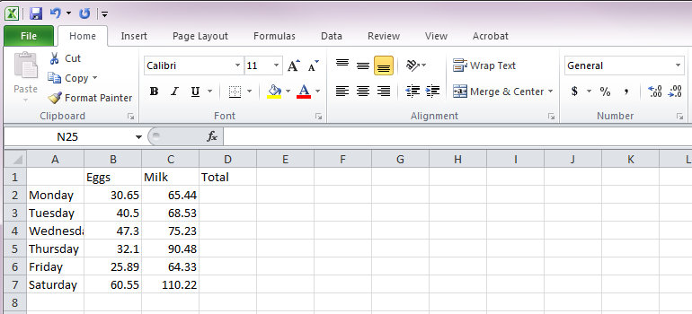
We can also format the entered data by selecting the '$' in the Number group. We can extend the formatting to the Total cells too. 

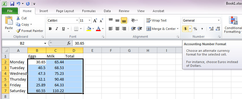
We can also widen column A so that all of Wednesday isn't clipped off. But finally, let's use a function!

In the Total column, we want the sum of the amount spent on eggs and milk. In cell D2 we type "=sum". As we type, Excel will give us a number of prompts for possible functions.

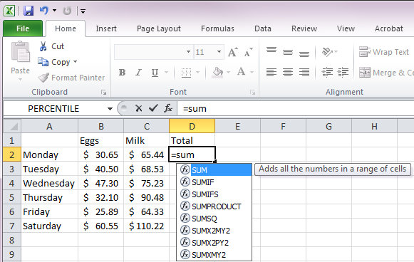
We're sticking to the basic sum function, so we'll continue by typing the open parenthesis. Then select cells B2 & C2 with the mouse (or by typing them).

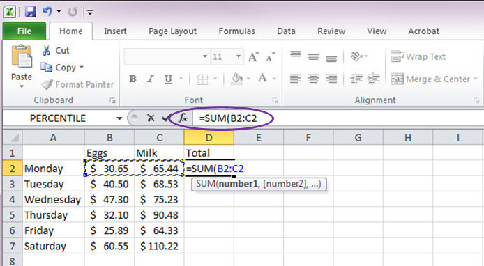
Notice that the function also appears in the formula bar. Then we can either type the ending parenthesis or simply press ENTER. Typically, we don't need to type the end parenthesis, because Excel will automatically add it for us, UNLESS we are writing a formula instead of using one Excel provides (or if we have a mistake in our argument list. We'll go over errors on the next page). After pressing ENTER we see this:

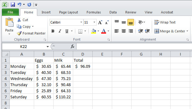
Using Auto Fill with Functions

Now we want to sum the information for the rest of the days. We can repeat what we just did: type "=sum(" and then select the cells, OR we can use Auto Fill. Remember that? Click on the cell with the function (in this case D2) and move the mouse over the bottom right corner until it makes a plus sign, and then click and hold down the mouse to select all the cells that you want to copy the function into. You'll see a gray outline showing the cells that are being selected. 

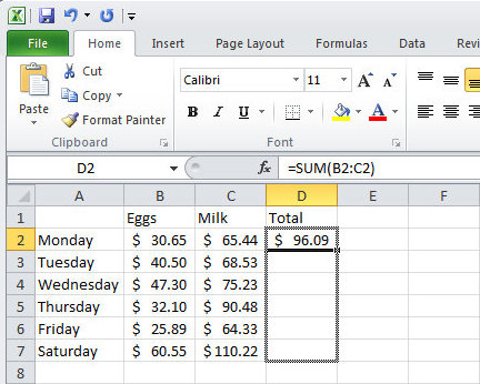
When you release the mouse, those cells will have the function copied into them, BUT changed to refer to the cells in each row. For example, look at D3 in the formula bar. 

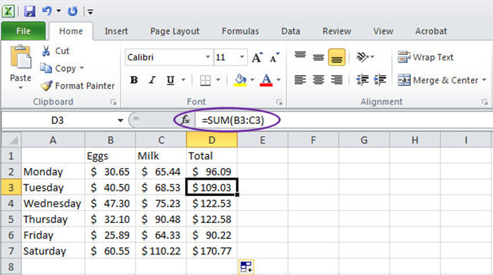
Essentially, Excel is copying: Dx = Bx + Cx, where x is the row number. You can also use Auto Fill horizontally. In this particular example, it doesn't make sense, but just to see how it works: select the cell with the function (in this case D2, again) and move the mouse over the bottom right corner to get the plus sign. Then click and hold the mouse down and drag to the right. You'll see the gray outline highlighting the selected cells. 

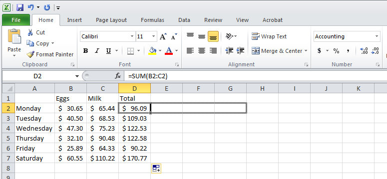
When you release the mouse, those cells will have the function. See E2 in the formula bar?

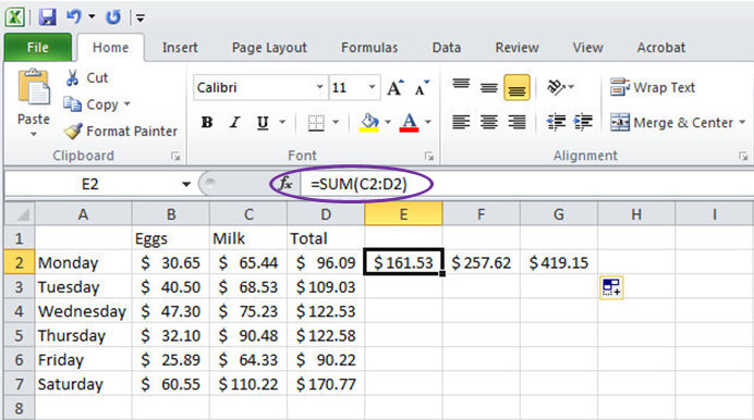
In this case, instead of copying: Dx = Bx + Cx, Excel is copying Y2 = (Y-2)2 + (Y-1)2, where Y represents the column letter and Y-1 represents one column letter to the left of Y, etc. To translate that- the columns change, not the rows. E2 is the sum of the cost of milk (C2) and the total cost of eggs and milk (D2), so in this dataset, summing this way makes absolutely no sense, but it is good to know how to do because there are datasets where it will make sense to Auto Fill horizontally instead of vertically. 

When I delete E2, I get this: 

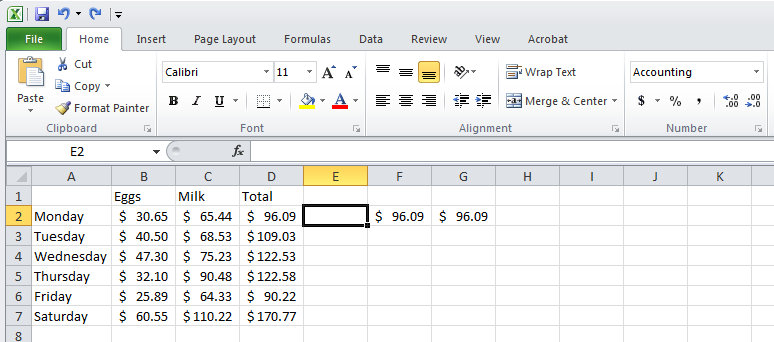
Can you figure out why $96.09 repeats in F2 & G2? Click here to find out if you are right. 

Finding Functions

For more possible functions, check out this external link to Microsoft which lists a variety of functions categorized based on their potential usage found in Excel 2010. 

Additionally, you can search for functions in Excel. Go to the Formula tab and you'll see a wide array of categories in the Function Library. Clicking on any of these categories will provide you with a list of related functions.

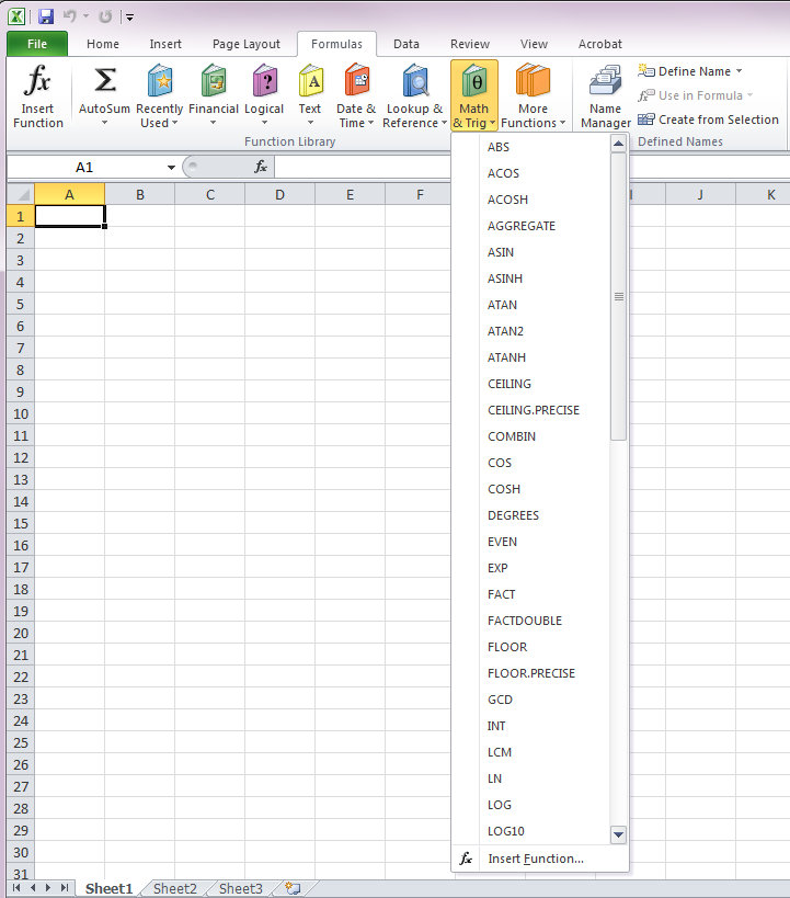
Since many of the functions are abbreviations, it isn't always clear what exactly they are. If you aren't sure what a function actually is, you can scroll over it and wait a second. A dialogue box will pop up and give you the details. 

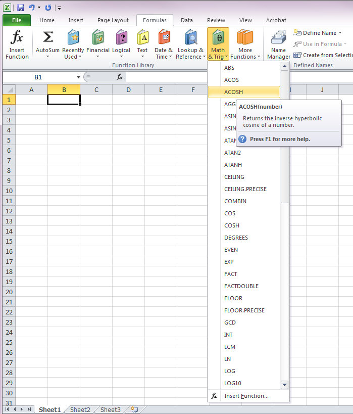
Who knew that we can use Excel to return the inverse hyperbolic cosine of a number?! Now we do!

You'll need to know the arguments necessary for each new function. This is presented in the parentheses. Even when Excel says that the function takes a number you can use a cell referent with a number, as opposed to entering the specific number. Remember all the reasons it is better to use a cell referent for a formula? (If not, go back to this page.) The same reasons apply to functions.

When you select the function in the dropdown menu from the previous step, (in this case we are looking at the ABS function which will give us the absolute value of a number) it will automatically open a dialogue box where you can enter the appropriate arguments. This can make navigating a new function much easier. 

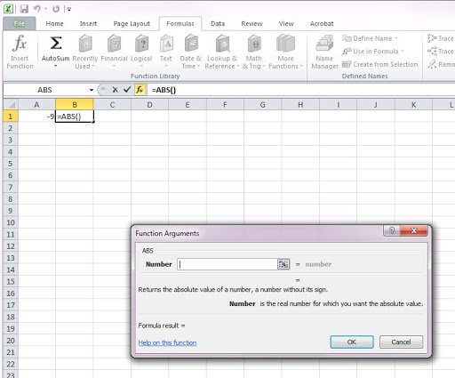
We are entering the function in cell B1 and will use cell A1 as the argument. You can either click on the cell or you can type 'A1' into the argument box.

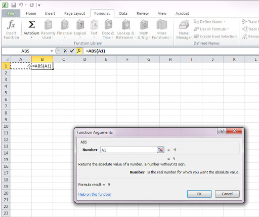
After clicking OK (or pressing ENTER) we get this:

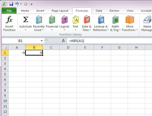
Notice that the function is visible in the formula bar when we click on B2, but the cell shows the output. As with writing formulas, if you want to edit the function, you can do so in the formula bar or by double clicking on the cell. 

And don't forget: no 'equals' equals no function!

Finding Functions

Finally, another way to track down a potential function is to use the Function Wizard. You can get to this by clicking on Insert Function to the far left in the Function Library group under the Formulas tab. One click will open this dialogue box:

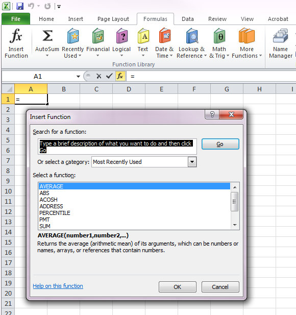
The '=' is automatically entered into the cell. You are given a list of functions under Select a function, but you can also search for a function by typing a brief description of what you want to do (in the first box that basically says what I'm typing here) and then clicking Go. 

I was thinking it would be nice to have a function that would only count instances of zero, so I search for 'count only zeros' and Excel offered me these options in the Select a function box: 

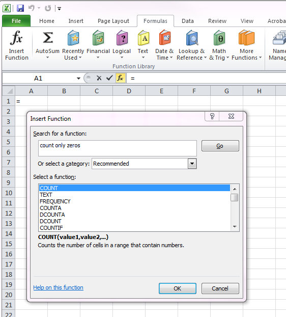
When you single click on a function, the required arguments and a description of what it does appears below the box. You can also get additional help with a function (if you are connected to the internet) by clicking on the Help with this function link in the bottom left corner. Once you decide on the function you want, click OK and it will open the Function Arguments dialogue box that we saw when we were exploring the ABS function above.

Which function do you think would best be able to count the number of zeros in a set of data? Click here to find out. 

As you might have noticed in the previous two pages (Formula Basics and Using Excel's Functions) there are a lot of commonalities between functions and formulas. These commonalities also extend to the possible error messages that may occur.

Some errors appear in a single cell and suggest some issue with the referents used in the formula or function. Other errors occur because of a typo or issue in the formula or function itself.

Cell Referent Errors

Dividing by Zero

You may have noticed this error in one of the cells in the previous example calculating the percent change in the Census 2010 dataset. 

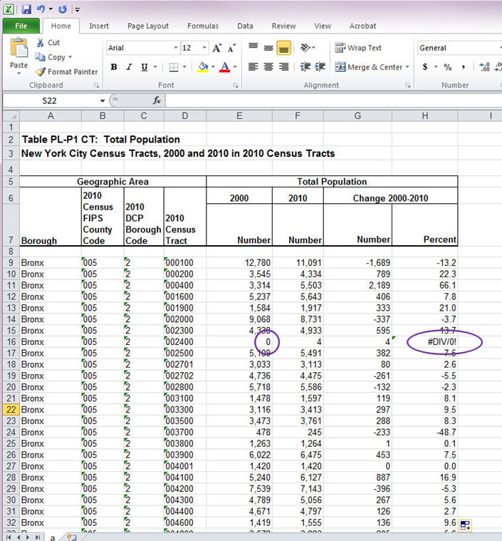
#DIV/0! means that you are trying to divide a number by zero which you can't do because the result is undefined. Since we can't do it, Excel can't do it either! So we get this error message. In this example, we can interpret what the error message means. The census tract in question didn't exist in 2000 so we can't measure the percent growth from 2000 to 2010. The original dataset used a dash (-) in cells where a new census tract was created. 

Cell Value Error

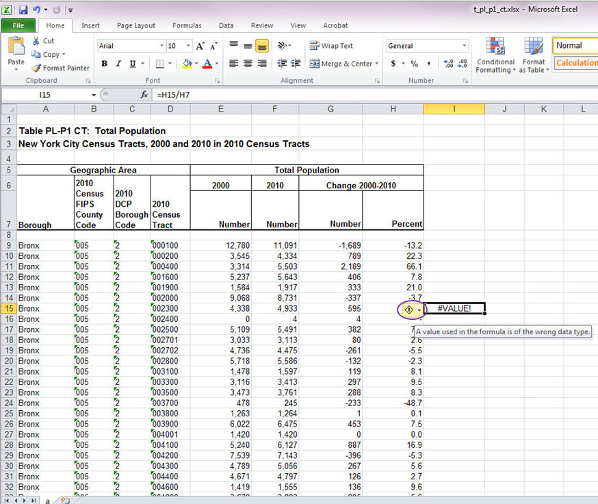
Another error message that can sometimes appear is #VALUE!

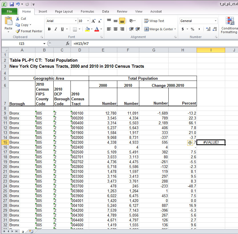
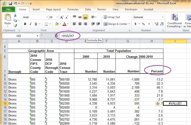
If we look at the formula bar, we see that someone (gee, I wonder who?) tried to divide information in cell H15 by information in cell H7. They must have made a mistake because what were the expecting to get dividing a number by text? What you get is this error message.

How to Fix an Error in a Cell

There are other error messages that can come up, but rather than trying to remember them all before they happen, you can learn about them when they appear. Notice that when we click on the cell with the error message that there is a small box with a yellow diamond and an '!' to the left of the cell. When we scroll the mouse over it an arrow appears, as does a text box explaining the error. 

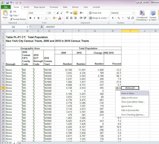
Furthermore, if the byline box doesn't clarify what the problem is, you can click on the arrow and get a number of options. 

Sometimes selecting Show Calculation Steps... will be enough to help you see where the mistake is.

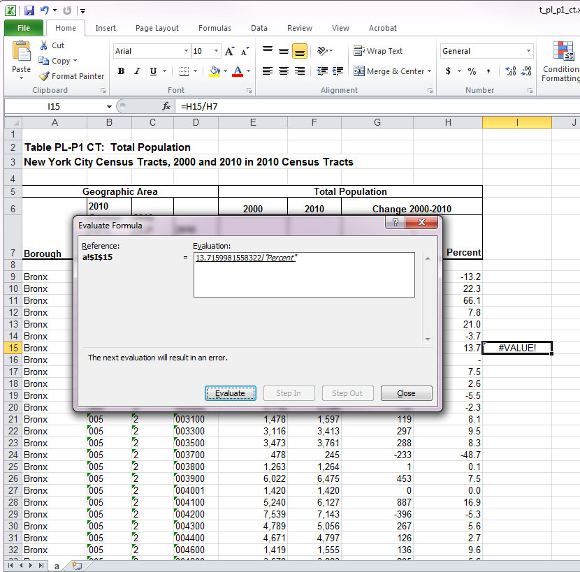
This person is trying to divide a number by text! How ridiculous!!!  But also easily resolved. 

Formula & Function Errors

While the previous errors are derived from the information in the cells referred to in the function or formula, other errors occur because of a problem in the function (or formula) itself. 

Circular Reference

It happens to the best of us. Sometimes when you are selecting a range of data for a function you misjudge where the dataset ends and quickly press ENTER. Then you see this:

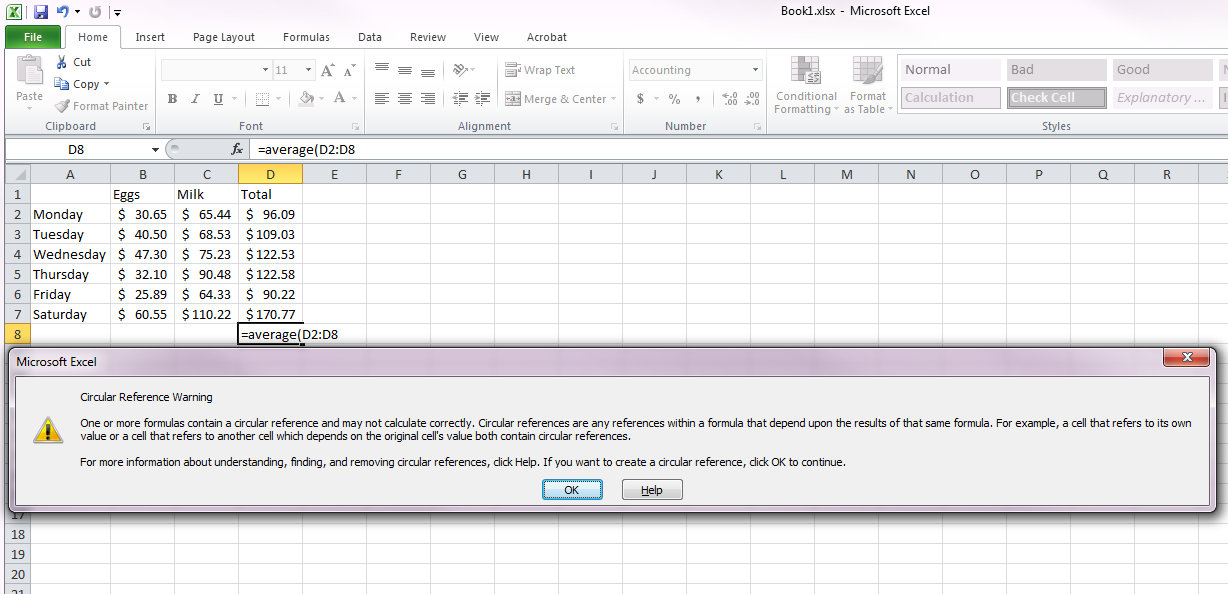
The range of data for calculating the average includes the cell (D8) where the average function is written. OOPS! By clicking OK Excel 2010 gives us this:

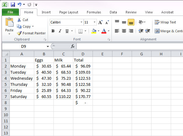
But this is easily remedied.
1. Click on the cell (D8) and edit the data range in the formula bar OR
2. Double click on the cell (D8) and edit the data range in the cell OR
3. Delete the function and start over- making sure to stop the range selection at D7 (or typing D2:D7).

Missing Parenthesis & Formula Errors

I know I've said previously in this tutorial that when using a function in Excel you do not need to type the ending parenthesis- and this is true, try it yourself!  But that doesn't mean the Missing Parenthesis error message doesn't pop up from time to time, and I'll show you some common issues that cause it. 

If you type a function and include no arguments, but press ENTER you'll get this:

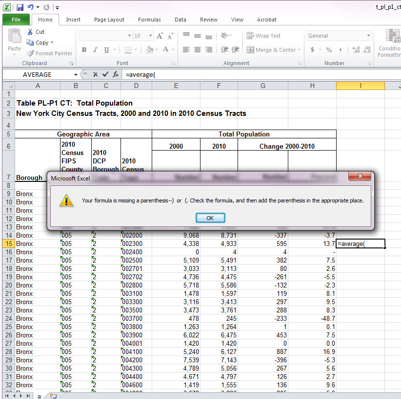
Even though the real problem is that the function contains no arguments, the error message is referring to the missing parenthesis. But since the error message recommends that you check the function, you'll see that there is more of a problem than just a missing parenthesis.

If your formula or function contains an error, and something you typed is inconsistent with Excel's syntax, you'll get the formula error message (even for functions).

In this example the average function was not given a number as an argument:

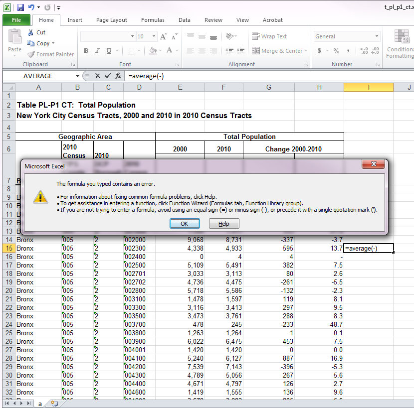
The error message offers suggestions that include checking out the Function Wizard. All magical entities are important to keep track of, so if you're not sure what it is, check it out here.

REMEMBER: A function, when given the correct arguments, doesn't need the ending parenthesis, but a formula does. A formula is something you write and a function pre-exists in Excel.

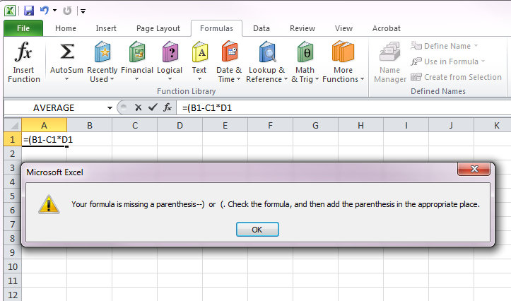
You would expect that the Missing Parenthesis error message would pop up if you are writing a formula that includes parentheses (for example, if you are adding or subtacting two numbers before multiplying or dividing them) and forget one end of the pair (either the open '(' or ending ')' parentheses), but check this out:

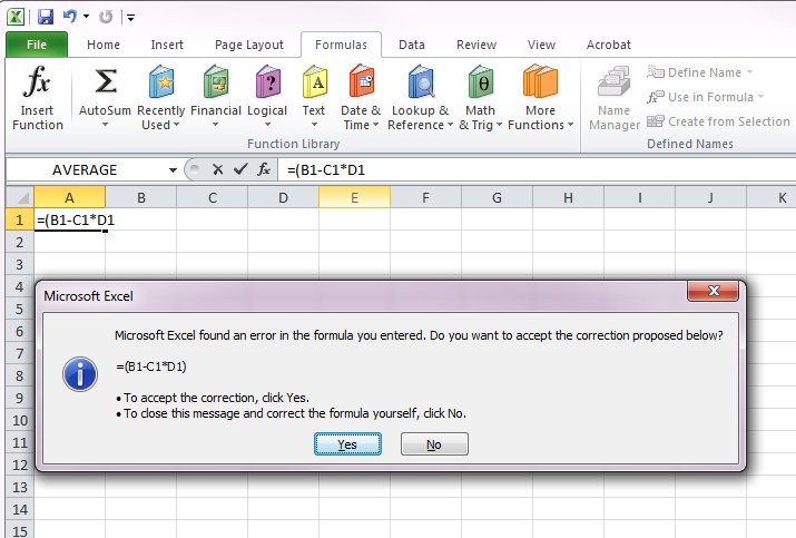
Instead Excel is helping us out by offering a proposed correction. Sometimes Excel's corrections are exactly what you want, but other times, like in this case, they miss the mark. 

CAUTION: Be wary that if you quickly press ENTER when seeing this message it will alter your formula, whereas, if you quickly press ENTER with the previous two error messages, they will give you the opportunity to edit your function. 

If you select NO to give yourself the option of editing the formula (which, in this case, you should), you will then get the Missing Parenthesis error message. 

Errors happen- it is a part of life and a potential side effect of being human. As long as you pay attention to the error messages that pop up, you will increase the accuracy of your data in Excel. 

However, there are errors that occur that Excel doesn't register, especially when manually entering data. Always be vigilant and double check, triple check, QUADRUPLE check your work!!

This page provides examples a few useful statistical functions you can use in Excel. Let's say you want to calculate two means, compare their standard deviations, and run a t-test to see if they're statistically distinguishable. 

Calculating the mean

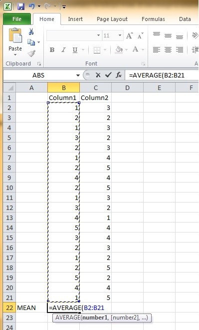
The AVERAGE function can calculate the mean of a distribution. Simply type "=AVERAGE(" and then fill in the column of numbers (which you can highlight as seen below). 

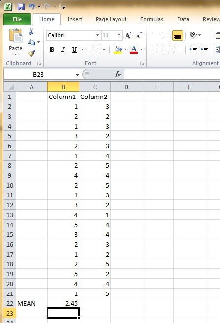
Then close the parentheses and hit enter. This will calculate the mean: 

You can click the cell and drag it over to calculate the mean for the next column as well:

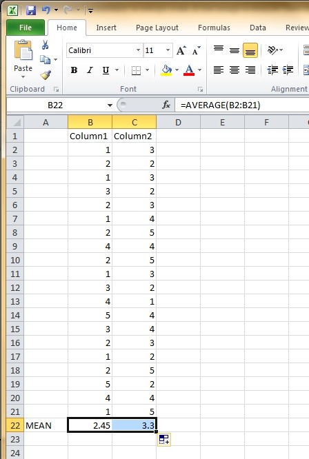
Now we see that Column1 has a mean of 2.45 and Column2 has a mean of 3.3.

Standard Deviation

You can get the standard deviation using the STDEV function. It uses the same logic as the AVERAGE function:

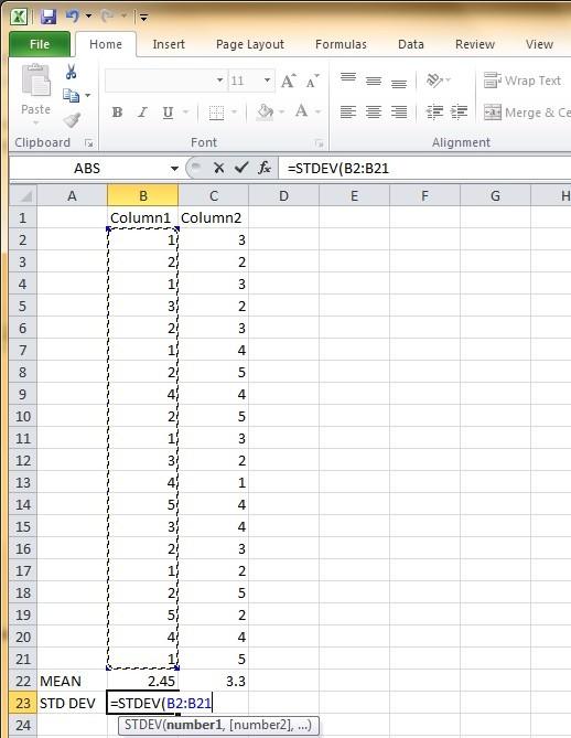
Close the brackets and hit enter to get the standard deviation for Column1. Then drag the cell to get the standard deviation for Column2 as well:

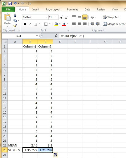
Column1 has a slightly larger standard deviation than Column2, but not by much. 

T-Test

Now we have some basic descriptive information about these two columns, but what about statistical significance? You can conduct a t-test in Excel using the TTEST function. This function requires four arguments. The first two are two arrays (columns or rows) you want to compare. The third argument is whether you want to use a 1- or 2-tailed test. Finally, the fourth argument is what type of t-test (Excel offers 3 options) you want. 

As seen below, we'll use B2:B21 as our first array and C2:C21 as our second array. Let's go with 2-tails and call for a type 2 t-test (more information about types can be found here):

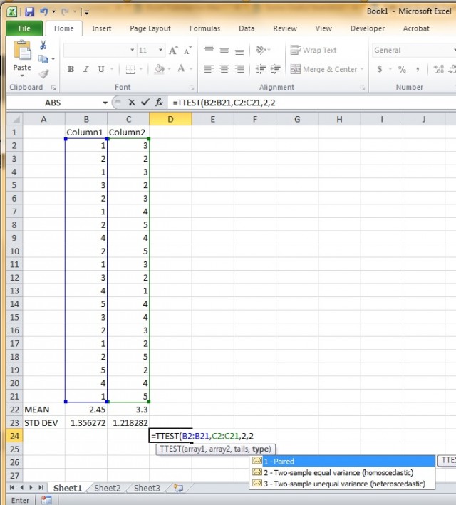
Close the parentheses and hit enter to get a p-value:

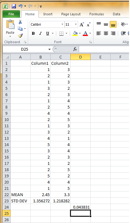
A p-value of .04 tells us this difference is statistically significant at the standard .05 level.

Why use Macros?

At its simplest, a macro is a recording of all of the commands and actions that you use to perform a complex task. A macro will let you repeat these tasks with a single click. Macros are stored as simple bits of code within Excel and they allow you to create complex functions, loop over entries in your spreadsheet, or quickly change formatting in your data. If you find yourself repeating the same set of tasks over and over again while dealing with a dataset, it can often be quicker to create a macro. One simple example of a macro is given here (for formatting text in cells), but macros can be used to format figures, clean datasets, or many other complex tasks. 

Getting Started

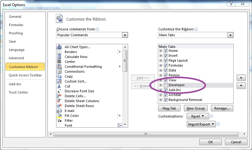
Before you can create your first macro, you need to activate the "Developer" ribbon in Excel. First go to File, and select Options. In the left panel, select Customize Ribbon and check the "Developer" box in the panel on the right and click OK. This will allow you to select the developer ribbon from the tabs at the top of the Excel window.

Recording Macros

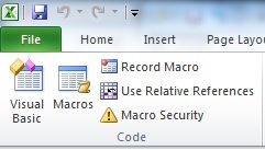
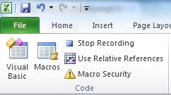
First, look at the options in the "Code" section of the Developer ribbon. 

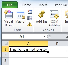
Select a cell in Excel you want to manipulate. As an example, we will create a macro that changes the font and formatting of text in a cell.

To record your macro, click the Record Macro button. This brings up a set of macro recording options. Here you can enter a name for your macro, a description for what it does, a keyboard shortcut, and specify where you would like to store it. Usually it is sufficient to store your macro in "This Workbook". This allows it to be used for the currently open spreadsheet. However, if it is something that you will use across many different datasets, you can save it either in a new workbook, or in a personal workbook that stores all of your macros on your computer. 

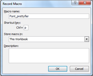
Once you have entered the name for you macro, click OK.This will bring you back to the spreadsheet. Perform whatever alterations to the dataset you wish to record. For our example, we will change the font, size, orientation (refresher on this here), and spacing of the text.

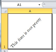
Once you are satisfied, return to the Developer ribbon and click the Stop Recording button. This will save your macro. The action required navigating 4 separate menus in Excel using multiple clicks. We can now repeat it for any cell with one click or keyboard shortcut.

Note: earlier in the tutorial we learned about using "$" before a cell entry to make an absolute cell reference versus a relative reference. By default, when you record a macro and refer to a cell value, it records that as an absolute reference. This means that if you run your macro again in a different position, it will always refer to the cell in the macro. By selecting "Use Relative References" you will be able to make your macros run using values relative to the cells where you are running it. 

Running your Macro

Clicking the Macros button will bring up a list of all of the macros you have stored.

Here you will see the full list of macros associated with this workbook. Selecting any macro and clicking Run will run the macro in the selected cell. If you assigned a keyboard shortcut when you named your macro, then you can also use the keyboard shortcut to activate your macro. 

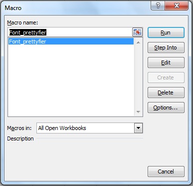
Macros are stored in a language called Visual Basic. Selecting Edit will allow you to edit the code for a macro. This can be a quick way to correct simple errors in a macro. If you wish to delete a macro, simply click Delete.

In a budget spread sheet, you put information about your budget, keep records of your monthly income and expense and come up with summary statistics for your monthly finance. By keeping clear transaction entries and making informative charts, you could have a better knowledge of your financial situation.

There are three separate sheets in this spread sheet: Income, Expenses and Statistics and Charts. 

Income

The first four columns of the income are self-explanatory and you just have to enter the transactions manually. We want the amount to show as currency instead of a plain number. To do this, we select the entire column and use the drop down menu in the Number section in the ribbon and then we select currency.

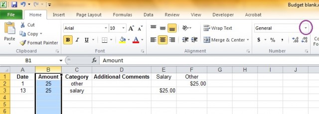
Throughout the whole budget spreadsheet, we will use currency for numbers. So if the default setting is “General”, we could simply select the whole range of numbers and change the form to currency.

Staring from column E, the column titles are different categories of income. In this example, we only have two categories of income: salary and other. You could specify other categories in column C and include the categories as different columns. We want the amount of income to be entered below certain categories starting from Column E without having to reenter the data in Column C. In order to do this, we use the IF function.

IF function

The IF function needs three arguments.

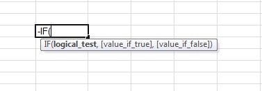
The logical_test is the condition you want to specify. For example, the condition for Column E would be if the entries have category as “salary”. So the condition for cell E2 would be: $C2=$E$1. Similarly, the condition for cell E3 would be $C3=$E$1. Note that the right hand side of the equation, we use absolute reference $E$1 for the entire Column E because we want to put any income that is categorized as “salary” in column C under Column E. (recall how to do absolute reference)

The next two arguments are [value_if_true] and [value_if_falso]. You specify what value to put into this cell if the condition is true or if it is false. In this case, you put nothing ("") in the cell is the category is not salary and put the amount of income ($B2) into the cell if the category is salary. So the full function statement for cell E2 would be =IF($C2=$E$1,$B2,""). The rest of the Column E can be auto-filled by dragging down the formula in cell E2. (Recall auto fill here)

The same idea applies for the column “Other”. We have the statement: If the category of the transaction specified in Column C is “other”, then put the amount under this column. Otherwise put nothing under this column. Then we translate the statement into the IF function. For example, the function in cell F2 would be: =IF($C2=$F$1,$B2, "").

Expense

In this sheet, we keep records of expenses. 

In addition to the date, amount, category, we also keep a record of whether this transaction is paid by cash. In Column D, we put “y” to indicate a cash transaction. After the normal bookkeeping columns, we have a column to count cash transaction and other columns to separate different categories of transactions. Again, we use IF function for this columns. In the “Cash Count” column, the if statement would be: if the corresponding record in column D for this transaction is “y”, then put the amount into column F, else put nothing. For example, the function in cell F2 would be: =IF(D2="y", B2, ""). In the following columns, we put the amount of transactions into the corresponding categories. The idea is very similar with that in the “Income” sheet. Note that we use red color to indicate negative number instead of putting a negative sign before the number. In order to do this, first select columns we keep information of the amount of money.

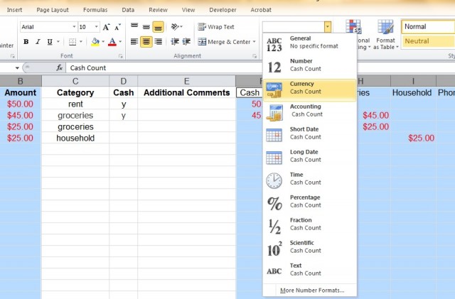
In this chart they are column B and columns after F. Then click the icon in the “Number” section of the ribbon. In the pop-up window, select the second option, which is using red color to represent negative numbers.

Statistics and Charts

Finally, we have the Statistics and Charts sheet to summarize our monthly budget and transactions. 

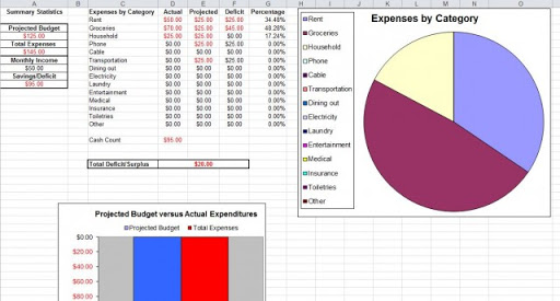
We first look at the middle part of this sheet, i.e. column C to G. These columns summarize expenses. In column C, we put different categories of expenses. Column D to G each gives the actual expense, projected expense, deficits of this category of expense and finally the percentage of total expenses which is used for this category. The projected expense is our budget and should be entered manually. The actual expenses come from the sheet “Expense”. For example, the total actual expenses for “Rent” would be the sum of all rental expenses, which is equal to the sum of entries in Column G of the Expenses sheet. In order to get the sum, we use the function SUM and we need to refer to cells in the expense worksheet. In order to do this, we write the command as: = SUM(Expenses!$G$2:$G$100). We actually only have four rows of transaction but we calculate the sum from row 2 to row 100 which also applies to larger data sets. For Groceries, similarly, we put =SUM(Expenses!$H$2:$H$100). Notice that we have to use absolute reference to cells and we cannot use auto fill for the following rows.

Why is this the case? Because if we use relative reference: = SUM(Expenses!G2:G100) and use auto fill for the following columns, the formula for the next row would be  = SUM(Expenses!G3:G101), which is not what we want.

After we calculated the actual expenses, we could calculate the deficit using actual – projected.  For example, F2=D2-E2, and we could auto fill the rest of the “Deficit” column. Having columns D, E and F filled out, we could calculate some numbers in Column A. Projected Budget is the sum of all numbers in Column E and Total Expenses are the sum of Column D. Then we could calculate Column G using the total expenses. Column G shows the percentage of each category of expenses to the total expenses. For example, cell G2 is calculated as: = D2/$A$6. Then we could auto fill the rest of the column.

The Cash Count would be the sum of amount of cash transactions, which is equal to: =SUM(Expenses!$F$2:$F$100). Total Deficit/Surplus shows the sum of Column F.

Now we could create some charts to summarize the calculated information.  We first make the projected budget versus actual expenditures chart. We first create a blank 2-D column clustered chart. Then we right click on the chart and choose “select data”.

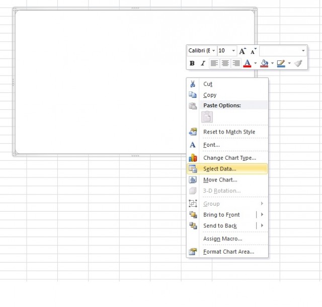
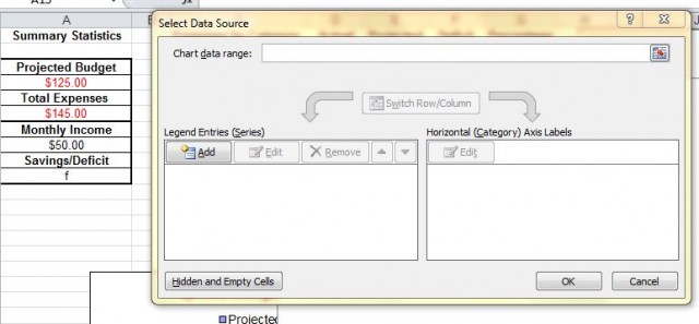
In the pop-up window and under the “Legend Entries”, we click on “Add”.  Then in the Edit Series window, choose cell A3 as the series name and cell A4 as the series value. Then click OK.

Similarly, add another series with A5 as series name and A6 as series value. After selecting the two legend entries, click OK.

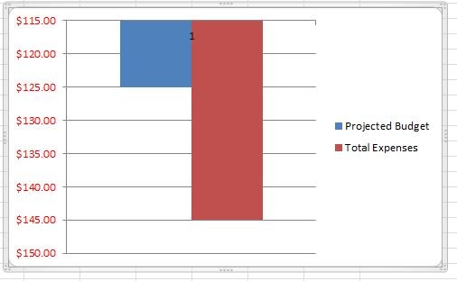
This is the chart you will get as a default. We could edit the chart to make it look better. We format the vertical axis to range from -150 to 0, move the legend to the top, and add a title for the chart. (Do not remember how to format a chart? Find various chart formatting tutorials here)

When you edit the chart, there is one tricky part that is worth mentioning. 

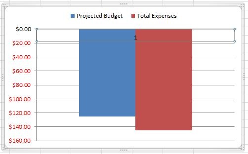
There is a small “1” between the two columns. To remove it, simply select it and press “Delete” on the keyboard. Note that it is very easy to select the actual “columns” or the whole chart area instead of selecting the number. Make sure that after you select the “1”, the chart area appears as in the picture above, otherwise you might want to try clicking on different positions on the chart.

Here is an example of a completed chart.

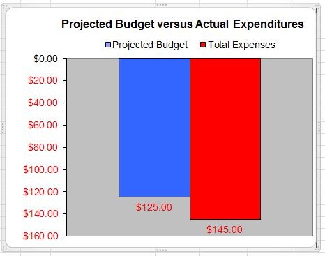
It is definitely fine to have other designs of the chart, as long as it is informative to you.

Then we make a pie chart to show expenses by category. Select Column C and D to include all categories of expenses and create a pie chart.

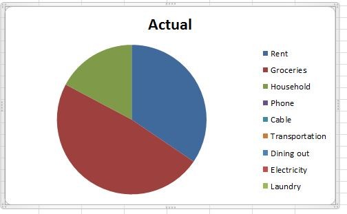
This will give you a default pie chart. Click on the title to edit it. You could also edit the legend and choose different style of chart area. Here is an example of the pie chart after some editing.

After summarizing the expenses, we could do similar analysis for income. 

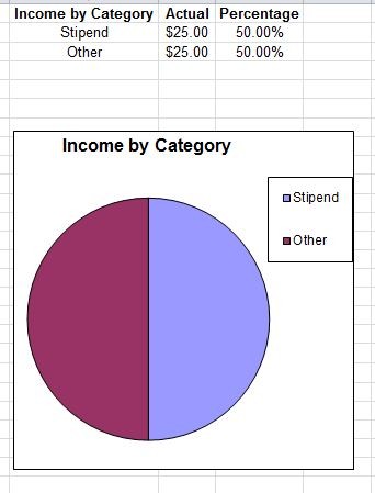
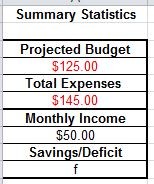
We copy the data from the Income spreadsheet using referencing another sheet to make the “Income by Category” and “Actual” columns. Then in the summary statistics in Column A, we calculate the monthly income by adding up all the income entries. We could also calculate Savings/Deficit, which is equal to the sum of total expenses (as a negative number) and monthly income.

Then we could calculate the percentage of each category of income by dividing the actual income by monthly income. We also make a pie chart to show income by category.

That is it! We have created a fairly informative budget spreadsheet.